There is a fundamental difference between knowing that a defect exists on a part and knowing exactly what that defect is: its size, shape, location, morphological class, and severity. The latter is what you need to make an intelligent, calibrated quality decision — one that distinguishes a 0.1mm surface pit from a 3mm structural crack, or separates a cosmetic blemish on a non-visible surface from the same blemish in a customer-facing area.
Bounding-box detection gives you the first level of information. Pixel-level segmentation gives you the second. This distinction is the key reason why AI visual inspection systems built on deep learning segmentation — rather than object detection — achieve lower overkill rates without sacrificing defect escape performance. This article explains how pixel-level classification works, why it enables threshold control that bounding boxes cannot support, and what that means for quality engineers managing FA/FR balance in production.
Key Takeaways
- Pixel-level segmentation assigns a defect class to every pixel in an image, providing exact defect area, boundary shape, and morphological type — not just a box around the defects.
- This granularity enables size-based and location-based threshold rules that bounding-box detection cannot support — the foundation of overkill reduction.
- Per-class threshold tuning is only possible with segmentation output: you can set zero tolerance for cracks while allowing minor cosmetic defects below a defined size to pass, all within the same inspection model.
- Labeling quality at the pixel level is the key determinant of model performance — the model learns exactly the boundaries it is shown during training.
The Limitation of Bounding-Box Detection
Bounding-box object detection — the architecture behind models like YOLO and Faster R-CNN — draws a rectangular region around a detected object and assigns it a class label and confidence score. For many computer vision tasks, this is sufficient. For manufacturing quality inspection, it creates a specific limitation.
Consider a scratch on an aluminum housing. The bounding box surrounds the scratch — but also includes a significant area of defect-free surface. The model outputs: “scratch detected, confidence 92%, at this location.” It cannot determine whether the scratch is 0.5mm or 5mm long, whether it crosses into a functional surface area, or whether it reaches the minimum size threshold in your defect specification. The confidence score provides no information about size or morphological.
As a result, every detected scratch above the confidence threshold triggers a rejection — regardless of whether it falls within cosmetic tolerance. To reduce overkill on small scratches, you lower the overall confidence threshold, which simultaneously increases the risk of missing larger scratches that the model returns with slightly lower confidence. You are tuning a single parameter that controls everything, with no way to distinguish severity.
Research published in the ASME Journal of Computing and Information Science in Engineering highlights this limitation: bounding-box detection cannot accurately measure crack width because detection occurs at the region level, whereas pixel-level localization provides the precision required for such measurements.
How Pixel-Level Segmentation Works
Pixel-level segmentation — specifically semantic and instance segmentation — assigns a class label to every pixel in the image. The output is not a box, but a mask: a precise boundary that traces the exact shape of each defect.
Semantic Segmentation
Semantic segmentation classifies each pixel into predefined categories: background, scratch, pit, crack, stain, and so on. The result is a pixel map where every pixel carries a class label. From this map, you can compute the exact area of a defect (number of defect pixels × pixel-to-millimeter conversion), as well as its orientation, aspect ratio, and location relative to defined functional zones.
Instance Segmentation
Instance segmentation extends this by distinguishing individual defect instances. If a part has three separate scratches, the output identifies three distinct masks rather than merging them into one region. This enables per-defect evaluation: scratch #1 is 0.3mm (acceptable), while scratch #2 is 4.1mm and crosses into a sealing surface (reject). Benchmarks, such as those from Roboflow, consistently show that instance segmentation outperforms object detection for manufacturing inspection due to its spatial precision.
What Pixel-Level Data Enables: The Threshold Architecture
With pixel-level segmentation output, quality engineers gain a rich set of parameters for defining acceptance criteria — per defect class, per part zone, and per severity level. This is what CorteX’s threshold interface is designed to leverage.
Size-Based Thresholds
Because segmentation provides exact defect areas, you can define rules such as: “Reject if scratch area ≥ 2.0 mm²” and “Accept if scratch area < 0.5 mm².” Parts falling between these thresholds can be routed to manual review. This tiered approach is not possible with bounding boxes, which lack reliable size measurements.
Location-Based Thresholds
Acceptability often depends on defect location. A pit on a non-sealing, non-visible surface may be acceptable, while the same pit on a sealing surface is a functional failure. Pixel-level segmentation identifies the exact position of each defect, — enabling zone-specific decision rules.
Morphology-Based Thresholds
Different defect types carry different engineering risks, even at similar sizes. A 1mm crack (linear, high stress concentration risk) is fundamentally more critical than a 1mm pit (localized, lower propagation risk). Pixel-level segmentation captures shape characteristics, such as aspect ratio, linearity, and edge sharpness — allowing the model to distinguish these morphologies and apply class-specific thresholds accordingly.
![]()
Bounding box detection (left) provides location and class, but no reliable size or morphology data. Pixel-level segmentation (right) provides precise defect boundaries, accurate area measurements, and exact location — enabling intelligent threshold rules that reduce overkill without compromising escape performance.
The Labeling Dependency: Why Training Data Quality Determines Threshold Precision
Pixel-level segmentation is only as precise as the pixel-level labeling used to train it. A model trained with rough, approximate defect boundaries will produce equally rough outputs at inference time — and size calculations derived from imprecise masks will be unreliable. This is not a theoretical concern; it is the most common root cause of threshold instability in AI inspection deployments.
Precise pixel-level labeling means: the annotator traces the true physical boundary of the defect, not an approximation inflated by a few pixels to ensure coverage. For defect types with clear edges — scratches, pits, and cracks on metal surfaces — this is achievable with standard labeling tools. For defects with diffuse boundaries — such as discoloration gradients, coating thickness variation, or subsurface inclusions visible through a translucent materials — boundary definition requires explicit labeling guidelines agreed upon by both the quality and AI teams before training begins.
CorteX’s labeling workflow includes structured quality checks for boundary precision — flagging annotations where the labeled boundary deviates significantly from the underlying image. This is critical because pixel-level labeling quality directly determines the threshold stability of the deployed model. For teams deploying AI inspection for the first time, the labeling review step often delivers the highest performance improvement per hour invested.
Overkill Reduction: The Practical Impact
The most direct operational impact of pixel-level threshold tuning is overkill reduction. Traditional rule-based machine vision systems are prone to false rejection rates of 5–15% or higher on variable parts — flagging legitimate surface variation, batch-to-batch texture differences, or reflectance changes as defects. Each false reject represents a good part unnecessarily scrapped or reworked, with full manufacturing cost invested.
At 10,000 parts per day, a 5% FR rate and a $20 part cost result in $10,000 per day in overkill — $3.6 million per year per line, before accounting for rework labor. AI inspection with pixel-level segmentation and properly tuned size thresholds consistently reduces FR to 1% or below on the same part types, recovering the majority of that cost while maintaining or improving FA performance on critical defects.
This is the quantified business case for pixel-level segmentation over bounding-box detection in manufacturing inspection — not a theoretical accuracy improvement, but a direct reduction in controllable yield loss. Explore how CorteX’s deep learning segmentation delivers this capability in production environments.
Pixel-Level Segmentation in Practice: What CorteX Provides
CorteX’s deep learning segmentation pipeline provides, for each inspected part:
- Defect class map: pixel-level classification of every defect region
- Defect location coordinates: precise position on the part surface for zone-based rule evaluation
- Part-level OK/NG decision: computed from all detected defects against the active threshold ruleset
This output is available at 100 MP/s inference speed — sufficient for high-speed inline production lines — and integrates with MES systems via 20+ supported industrial protocols for real-time data traceability and closed-loop quality control. The Central Management System stores threshold rulesets per part number, enabling instant rule activation during product changeovers without re-programming the inspection station.
Comparison: Bounding Box Detection vs. Pixel-Level Segmentation for Threshold Control
| Capability | Bounding Box Detection | Pixel-Level Segmentation (CorteX) |
| Defect presence detection | ✓ Yes | ✓ Yes |
| Defect class identification | ✓ Yes (per box) | ✓ Yes (per pixel) |
| Precise defect area measurement | ✗ No (box includes background) | ✓ Yes (pixel count × conversion) |
| Size-based threshold rules | ✗ Not reliable | ✓ Fully supported |
| Zone-based tolerance rules | ✗ Approximate only | ✓ Pixel-precise location |
| Morphology distinction (crack vs. pit) | Partial (shape of box only) | ✓ Full shape and aspect ratio data |
| Overkill reduction on cosmetic defects | Limited — no size data to exclude small defects below tolerance | ✓ Precise size thresholds eliminate overkill on sub-tolerance defects |
Frequently Asked Questions
What is pixel-level defect classification in AI visual inspection?
Pixel-level defect classification — or deep learning segmentation — is an AI technique that assigns a defect class label to every pixel in an inspection image, rather than drawing a bounding box around a defect region. The output is a precise mask that traces the exact boundary of each defect, providing size, shape, location, and morphological class. This granular output enables intelligent threshold tuning — allowing the inspection system to distinguish a 0.2mm scratch (potentially acceptable) from a 5mm crack (reject), based on measured defect properties rather than a single confidence score.
Why does pixel-level segmentation reduce overkill compared to bounding box detection?
The overkill problem in bounding-box detection stems from its inability to distinguish defect size: all detected defects above a confidence threshold trigger a rejection, regardless of actual size. Pixel-level segmentation provides exact defect area, enabling size-based threshold rules: defects below a defined size threshold can be automatically accepted without affecting rejection decisions for larger defects of the same class. This is what reduces FR (overkill) without increasing FA (escape risk) on critical defects — the core mechanism behind overkill reduction in pixel-level systems.
Does pixel-level segmentation work at production line speeds?
Yes. CorteX’s segmentation inference engine runs at up to 100 MP/s — sufficient for high-speed production lines operating at up to 1,200 parts per minute, depending on part size and field of view. Segmentation, including defect area calculation and threshold evaluation, is completed within the inspection cycle time without requiring line speed reduction. This is why CorteX’s deep learning inference is engineered for edge deployment — processing occurs directly at the inspection station, not in a cloud round-trip.
How do I define defect tolerance zones on a part for zone-based threshold rules?
Zone definitions are configured in CorteX as a part reference layer — a mapped overlay on the nominal part image that designates functional zones (zero tolerance), cosmetic zones (size-based tolerance), and non-visible zones (liberal tolerance). These zone definitions are created once per part number during initial model setup and stored in the Central Management System. On product changeover, the correct zone map is activated automatically alongside the part-specific AI model.
Learn more about CorteX deep learning segmentation — or talk to UnitX experts to see pixel-level threshold tuning in action on your specific part and defect types.