When a defect is the size of a single pixel — a hairline crack in a battery tab or a pinhole in a connector coating — a classification label is not enough. You need to know exactly where it is, what shape it takes, and how far it spreads. That demand is precisely why Fully Convolutional Networks (FCN) became a foundational architecture in modern machine vision. Unlike conventional neural networks that collapse spatial information into a fixed-size output, an FCN preserves the geometry of the image from input to output, enabling pixel-by-pixel decision-making at production-line speed. This guide explains how FCN works, where it outperforms other approaches, and what it means for AI-powered industrial inspection today.
Key Takeaways
- FCNs replace fully connected layers with convolutional layers, enabling pixel-level predictions on images of any size.
- In industrial inspection, FCNs enable deep learning segmentation that maps the exact boundary and shape of each defect — not just a bounding box.
- Modern AI visual inspection systems combine FCN-derived architectures with generative training tools to achieve near-zero defect escape rates, even when training data is limited.
What Is a Fully Convolutional Network?
The Core Architecture Shift
A standard Convolutional Neural Network (CNN) ends with one or more fully connected (dense) layers that reduce the entire feature map to a fixed-size vector — useful for classifying an image as “defective” or “good,” but insufficient for locating where a defect exists. A Fully Convolutional Network eliminates those dense layers entirely. Every layer is convolutional, allowing the network to retain spatial coordinates throughout the computation pipeline.
The landmark paper by Long, Shelhamer, and Darrell — “Fully Convolutional Networks for Semantic Segmentation” (CVPR 2015) — demonstrated that replacing dense layers with 1×1 convolutions enables a trained classification network to produce a spatial output map with resolution proportional to the input. This insight transformed computer vision from image-level reasoning to pixel-level reasoning.
Downsampling and Upsampling: How FCN Sees at Multiple Scales
FCNs use two complementary mechanisms to handle scale. Pooling layers progressively reduce spatial resolution, compressing information into abstract feature representations — this is the encoder path. Upsampling layers (transposed convolutions, bilinear interpolation, or skip connections) then restore the resolution back to the original image size. This combination allows the network to capture both fine-grained texture (small defects) and broader spatial context (defect location relative to part geometry).
The FCN-8s variant, introduced in the original paper, uses skip connections from earlier pooling layers to feed high-resolution detail back into the upsampling path. In a 2019 IEEE Access study on pixel-wise surface defect detection, an FCN-8s configuration achieved 92.25% segmentation accuracy on industrial test images, compared to 79.35% for FCN-32s — demonstrating how skip connections improve spatial precision, as detailed in the study “A High-Efficiency Fully Convolutional Networks for Pixel-Wise Surface Defect Detection.”
FCN vs. CNN: When Segmentation Beats Classification
The Localization Gap
Standard CNNs answer the question: “Is there a defect?” FCNs answer: “Where is every defective pixel, and what does it look like?” For go/no-go quality gates on a production line, classification may appear sufficient. But the moment an engineering team needs to distinguish a 0.3 mm scratch from a 0.8 mm gouge — because one triggers rework and the other triggers scrap — only pixel-level segmentation provides the spatial measurement data required.
| Attribute | Standard CNN (Classification) | FCN (Segmentation) |
| Output | Single label per image | Label per pixel |
| Spatial information retained? | No — collapsed to vector | Yes — full resolution output |
| Input image size flexibility | Fixed size required | Any size accepted |
| Defect boundary measurement | Not possible | Pixel-accurate boundary map |
| Typical use in quality inspection | Binary pass/fail gate | Defect sizing, classification, and grading |
| Inference speed (relative) | Fast | Fast to moderate (architecture-dependent) |
FCN Variants Used in Industrial Inspection
The original FCN has spawned a family of architectures that are now standard in production inspection systems:
- U-Net: Adds symmetric skip connections between the encoder and decoder. Particularly strong for defect segmentation with limited training data. In a 2025 benchmark study on component segmentation, U-Net achieved 80.3% accuracy with an IoU of 85.8 — outperforming vanilla FCN (77.7% accuracy) on the same dataset (per Nature Scientific Data, 2025).
- DeepLabV3+: Uses dilated (atrous) convolutions to expand the receptive field without additional pooling. This allows it to capture large-area defects without sacrificing fine boundary detail.
- SegNet: Uses pooling indices from the encoder to guide upsampling, reducing memory requirements — valuable for edge deployment in embedded inspection hardware.
How FCN Enables Deep Learning Segmentation in Manufacturing
Pixel-Level Defect Detection in Practice
Consider a connector terminal inspection task. A traditional rule-based vision system defines zones and brightness thresholds — it flags anything outside those parameters. A scratch within tolerance? Flagged. A good part with minor lighting variation? Flagged. The result is a high False Rejection Rate (FR) and frequent operator overrides.
An FCN-based system learns the visual semantics of each defect type from labeled training images. Instead of relying on rules, it builds internal representations of what a true scratch, a true dent, and a true contamination look like — at the pixel level. The network outputs a segmentation map where every pixel carries a defect class probability. Quality engineers can then set grading thresholds based on defect area, aspect ratio, or location relative to functional zones.
In a 2026 study published in the International Journal of Computer Information Systems and Industrial Management Applications, an FCN-8s model deployed on a robot vision inspection system for industrial workpieces (bearings, gears, wrenches) achieved 98.30% average pixel accuracy — a 15.97% improvement over traditional template-matching methods, along with inference speed gains of 83–84%.
Two-Stage FCN Frameworks for Efficiency
A two-stage FCN approach — using a lightweight FCN for initial region proposal and a second, more precise FCN for fine segmentation — offers a practical speed-accuracy trade-off. Research from the Harbin Institute of Technology demonstrated this pattern in industrial surface defect inspection: the lightweight segmentation stage runs at sub-100ms latency, filtering the image to candidate defect regions before the precision network applies detailed analysis only where needed (per ResearchGate, “Fully Convolutional Networks for Surface Defect Inspection in Industrial Environment”).
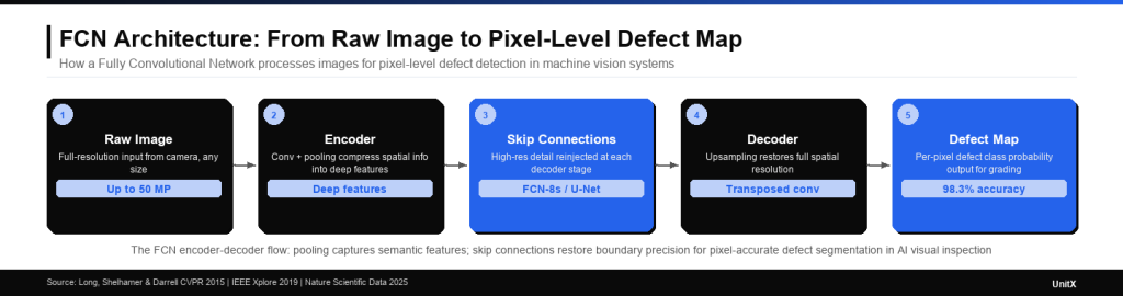
The FCN encoder-decoder architecture compresses spatial information and then restores it through upsampling — with skip connections feeding high-resolution detail back at each stage. This flow explains why FCNs can locate defects at pixel-level precision without losing the broader context needed to classify them.
FCN and the Semiconductor Wafer Inspection Challenge
Why Wafer Maps Demand Pixel-Level Intelligence
Semiconductor yield management is one of the most demanding segmentation applications. Wafer defect maps encode spatial patterns — edge rings, center clusters, and scratch lines — that indicate specific process failures. A 2026 comparative study from the Asian Journal of Applied Research and Reviews evaluated FCN, SegNet, and U-Net on synthetic wafer map defect patterns using Intersection-over-Union (IoU) as the primary metric. The study concluded that while FCN provides a computationally efficient baseline, U-Net and SegNet outperform it when defect boundaries are irregular — a finding that supports using FCN-derived architectures rather than vanilla FCN for high-mix semiconductor inspection (per ResearchGate, Balachandar Jeganathan, 2026).
For manufacturers in the semiconductor space, this translates into a clear system design principle: the FCN architecture provides the foundation for spatial prediction, but the specific variant — U-Net for thin-film layer defects, DeepLabV3+ for large-area pattern analysis — should be selected based on the defect morphology at each process step. Exploring UnitX’s semiconductor inspection solutions illustrates how this principle is applied in production-grade deployments.
Training an FCN: Data Requirements and the Labeling Problem
Why Pixel-Level Labeling Is the Bottleneck
The greatest operational challenge in deploying FCN-based inspection is not model architecture — it is labeled training data. Pixel-level labeling (also called semantic labeling) requires a human expert to trace the boundary of every defect instance in every training image. For production defects with irregular, fractal-like geometry, this process can take minutes per image. At scale, it becomes a significant project cost.
Two strategies help reduce this burden. First, transfer learning: initialize the FCN with weights from a large-scale vision dataset (e.g., an ImageNet-pretrained ResNet backbone), then fine-tune on domain-specific defect images. A 2024 study in the International Journal of Advanced Manufacturing Technology showed that FCNs using transfer learning achieved F1 = 0.94 for metal surface defect detection — compared to F1 = 0.52 for networks trained from scratch on the same small dataset.
Second, synthetic data augmentation: generate photorealistic defect images using generative AI tools to supplement real labeled images. This approach is particularly valuable when rare defect types — those that occur once per thousand parts — cannot be captured in sufficient volume through production sampling alone.
Minimum Training Requirements for Industrial FCN Deployment
| Training Strategy | Min. Labeled Images | Expected Accuracy | Best Use Case |
| Train from scratch | 1,000–5,000+ | Moderate | High-volume, single defect type |
| Transfer learning | 50–200 | High | Multi-defect, limited data |
| Transfer + synthetic augmentation | 5–50 real images | High to very high | Rare defects, new product introduction |
The “transfer + synthetic augmentation” approach — combining small real datasets with AI-generated defect images — is how systems like UnitX’s FleX-Gen generative AI tool reduce the labeling burden for production FCN model training. With as few as 3 real defect images, FleX-Gen can synthesize a full training set — reducing false rejection rates by up to 9× compared to models trained on real data alone.
FCN in Production: Integration with Real-Time Inspection Pipelines
Latency and Throughput Requirements
An FCN model running inference on a 50 MP image requires hardware that can keep pace with production cycle time. For a line running at 1,200 parts per minute — a realistic target for connector or EV battery tab inspection — the system must complete image capture, preprocessing, FCN inference, and defect classification within roughly 50 milliseconds per part.
Modern AI inference hardware achieves this through two mechanisms: GPU parallelism (processing thousands of pixel predictions simultaneously) and model optimization (quantization, pruning, or distillation to reduce compute requirements without significant accuracy loss). When CorteX is configured for high-throughput inspection, it processes images at up to 100 megapixels per second — sufficient for multi-camera, multi-angle FCN inference at full production speed.
From FCN Output to Quality Decision
The raw output of an FCN is a probability map: each pixel carries a confidence score for each defect class. Converting that map into an actionable quality decision requires post-processing logic: thresholding, connected-component analysis (to count and measure individual defect instances), and rule application (e.g., defect area greater than X mm² and located within critical zone Y triggers reject signal). This post-processing layer is where engineering judgment translates pixel-level AI output into manufacturing process control — feeding real-time data into the MES for closed-loop quality management.
If you are evaluating AI visual inspection systems for a production line and want to see how FCN-based deep learning segmentation performs on your specific part geometry and defect types, contact the UnitX team to discuss a proof-of-concept deployment.
Frequently Asked Questions
What is the difference between FCN and CNN in machine vision?
An FCN produces a spatial output map (one prediction per pixel), while a CNN with fully connected layers produces a single output vector (one prediction per image). In machine vision, this means FCNs can locate and measure defects at pixel-level resolution, while standard CNNs can only classify whether a defect exists somewhere in the image. For industrial inspection tasks requiring defect sizing or boundary measurement, FCNs — or their derivatives, such as U-Net — are the appropriate architecture.
How much training data does an FCN need for industrial defect inspection?
With transfer learning from a pretrained backbone, production-grade FCN models can be trained with as few as 50–200 labeled images per defect type. When synthetic data augmentation is added — using generative AI to create additional training images from a handful of real examples — that requirement decreases further. The critical constraint is not total image count, but the diversity of defect morphologies and imaging conditions represented in the training set.
Can FCNs handle images of different sizes in a production inspection system?
Yes — this is one of FCN’s defining advantages over architectures with fully connected layers. Because every layer is convolutional, an FCN can process input images of varying spatial dimensions. This is particularly important in production systems where camera resolution or field of view may change between product changeovers, or where the system must inspect parts of different sizes without retraining the model.
Is an FCN faster than object detection models like YOLO for defect detection?
It depends on the task. YOLO-family models are optimized for bounding-box detection and run extremely fast on objects with well-defined boundaries. FCNs (and U-Net variants) are optimized for pixel-level segmentation and typically require more computation per image — but they deliver much richer spatial information. For defects where boundary shape and area matter (e.g., cracks, corrosion patches, delamination), FCN-derived segmentation is the correct choice despite slightly higher latency. For simple presence/absence detection of well-defined objects, detection models may be faster.
How does UnitX use FCN in its AI visual inspection system?
UnitX’s CorteX system uses deep learning segmentation — built on FCN-derived architectures — to measure the exact pixel-level shape and boundary of each detected defect. This enables defect grading (not just pass/fail), dimensional measurement of defect geometry, and root-cause traceability through the MES. Combined with the OptiX multi-angle imaging system and FleX-Gen synthetic data generation, CorteX delivers what legacy rule-based vision systems cannot: adaptive, sample-efficient AI inspection that improves as production data accumulates. View customer case studies to see FCN-based inspection results across automotive, battery, and semiconductor applications.