Most quality teams recognize that manual inspection and legacy rule-based vision systems have a hard ceiling. Human inspectors are prone to fatigue, while rule-based systems struggle with normal product variation Today, the question most production engineers ask is not whether to adopt AI visual inspection: it is how to deploy it without disrupting live production or wasting months of engineering time. This guide answers that question with a five-phase framework drawn from real deployments across automotive, battery, and semiconductor manufacturing lines.
Key Takeaways
- A structured five-phase approach: audit, data collection, AI training, site acceptance testing, and production rollout, is the fastest path from decision to live inspection.
- Data collection quality is the single most predictive variable of AI model accuracy; 50+ labeled images per defect class is the minimum viable dataset.
- Site Acceptance Testing (SAT) with live production parts, targeting a False Acceptance Rate (FA) = 0% and False Rejection Rate (FR) ≤ 1%, is non-negotiable before full deployment.
- MES integration enables real-time data traceability and closes the quality control loop from day one of production.
- Synthetic defect generation via generative AI significantly reduces the data collection burden for rare defect classes.
Why AI Visual Inspection Is No Longer Optional in 2026
The business case has matured. According to a McKinsey Global Institute analysis, manufacturers that adopt AI-driven quality control outperform peers on defect escape rates by a factor of 3–5x within two years of deployment. Meanwhile, NIST research on AI adoption in manufacturing confirms that the primary barrier is not technology readiness, it is implementation methodology.
The 2026 landscape differs from 2022 in three important ways:
- Advanced Illumination: Software-defined imaging systems now offer 32-channel independent lighting control, enabling reliable inspection under conditions that were previously impossible to standardize.
- Sample-Efficient Deep Learning: You no longer need thousands of defect examples to train a production-ready model. Modern AI training systems, like CorteX, can begin with as few as five labeled images per defect class.
- Synthetic Data Generation: Generative AI tools can now synthesize realistic defect images for rare defect categories, eliminating the traditional catch-22 of needing to train a system on defects your line rarely produces.
Phase 1. Line Audit: Define the Problem Before Touching Any Technology
What to Measure in Your Audit
A line audit is not a factory tour. It is a structured data-gathering exercise with a specific output: a defect taxonomy paired with throughput and cycle time (CT) constraints that the AI system must satisfy. Every defect class must be named, photographed under production lighting, and ranked by frequency and severity. If you engage an AI vendor without this taxonomy in place, you will spend the first month of the project performing the audit anyway, at significantly higher cost.
The audit should document: all defect types and their approximate occurrence rates; the physical dimensions and surface textures of parts under inspection; current cycle time (CT) and the maximum inspection CT the line can absorb; downstream MES schema and communication protocols; and any regulatory or traceability requirements (ISO 9001, IATF 16949, etc.).
Why Lighting Decisions Happen in Phase 1
Lighting is the most underestimated variable in AI visual inspection. Inconsistent illumination produces image variation that the model must learn, inflating data requirements. A software-defined imaging approach, where each illumination channel is independently controlled and reproducible, eliminates this variability at the source. Define your illumination architecture during the audit, not during model training, or you will need to retrain when lighting changes.
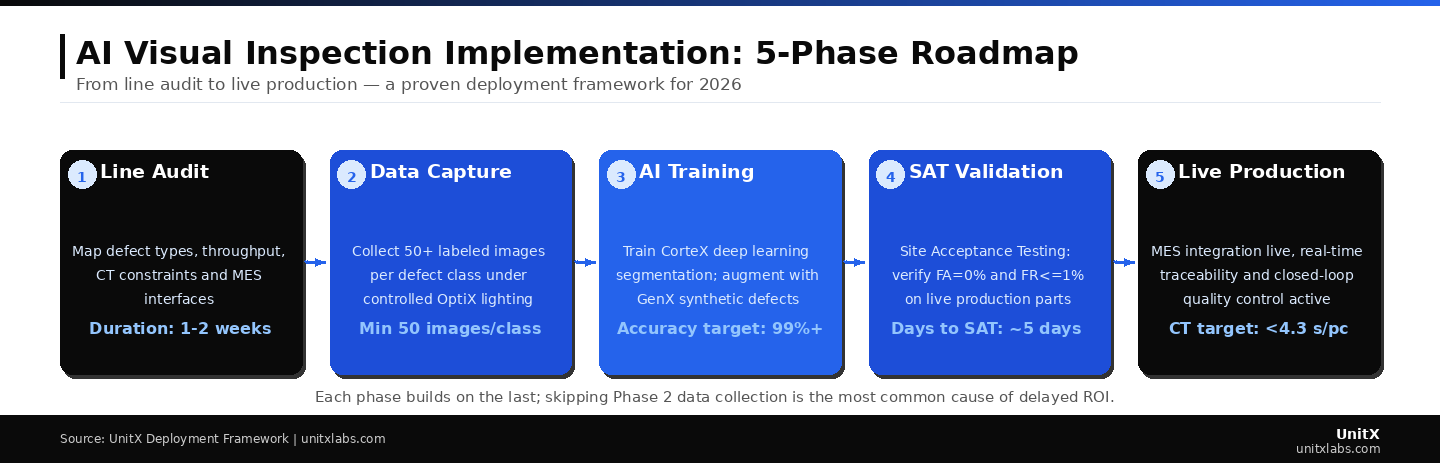
Each phase builds on the last; skipping Phase 2 (data collection) is the most common cause of delayed ROI. Cycle time targets and SAT thresholds must be defined in Phase 1 to ensure correctly in Phase 4.
Phase 2. Data Collection: The Make-or-Break Stage
The 50-Image Rule and When to Break It
Fifty labeled images per defect class is the practical minimum for training a reliable deep learning segmentation model on industrial parts. Below this threshold, model generalization typically degrades when surface finish or lighting varies between shifts. Above 200 images per class, accuracy improvements per additional image diminish rapidly. The goal is not maximum data, it is representative data.
For rare defects, catastrophic failures that may appear only once per thousand parts, generative AI fills the gap. By training a generative model on the limited real examples available, you can produce statistically plausible synthetic defect images that expand your dataset without waiting months for real defects to accumulate. UnitX FleX-Gen is purpose-built for this use case, reducing false rejection rates by up to 9× compared to models trained on real data alone.
Labeling Standards That Survive Model Updates
Every image must be labeled in a way that is unambiguous, repeatable, and strictly aligned with the defect taxonomy established in Phase 1. The labeling process should document the part ID, defect class, image acquisition parameters (lighting channel settings, distance, angle), and the inspector responsible. This metadata becomes critical during Phase 4 validation, when you need to trace any model error back to a specific data source. IEEE quality data standards for machine learning provide a useful framework for establishing labeling governance.
Phase 3. AI Model Training: Getting to 99%+ Accuracy
Deep Learning Segmentation vs. Classification
For industrial defect detection, deep learning segmentation, where the model identifies the exact pixel-level boundary of a defect, outperforms simple classification on every production-relevant metric. Classification tells you whether a defect exists; segmentation tells you where it is, how large it is, and whether it crosses a dimensional threshold. This distinction is critical when quality specifications define defects by size (e.g., scratch length ≥ 0.3 mm constitutes a reject).
Training on modern inference hardware can reach speeds of up to 100 megapixels per second, meaning a full training cycle on a well-curated 5,000-image dataset can complete in hours rather than days. The critical output of Phase 3 is not just a model, but a model card documenting accuracy by defect class, the confidence thresholds used, and known failure modes.
Setting Acceptance Thresholds Before Training
Many teams make the mistake of training a model first and evaluating accuracy afterward. The correct sequence is the reverse: define acceptance thresholds first, then train until the model meets them. For most production applications, FA (False Acceptance Rate) = 0% is non-negotiable. A defective part reaching the customer is a quality escape with direct liability implications. FR (False Rejection Rate) ≤ 1% is typically the economic target; above 5%, overkill scrapping begins to affect yield economics. ISO 9001:2015 Section 8.5.1 provides the framework within which these thresholds are documented.
Phase 4. Site Acceptance Testing: Proving the System on Your Parts
What a Proper SAT Looks Like
Site Acceptance Testing (SAT) verification that the AI visual inspection system meets specification on your actual production line, not in a lab, not on benchmark parts, but on real production output at full throughput. A well-run SAT typically takes about five days and produces documented evidence across three dimensions: inspection accuracy (FA=0%, FR ≤ 1%); cycle time compliance (CT meets the constraint defined in Phase 1); and system integration (MES communication confirmed, alarm handling verified, and data logging validated).
The five-day SAT benchmark is achievable with systems that use pre-trained deep learning inference rather than rule-based programming. Legacy systems often require three to six weeks of tuning per product changeover. Real-world deployment case studies show that AI inspection systems consistently achieve SAT in days rather than weeks due to their generalization capability.
Handling Product Changeovers
A common question during SAT planning is how the system handles product changes. In rule-based systems, new products requires new rules, effectively a new system. In deep learning systems, changeovers require only additional labeled images and retraining, typically completed in under 48 hours with a well-maintained dataset pipeline.
Phase 5. Live Production: Closing the Quality Loop with MES Integration
Real-Time Data Traceability
Going live is not the end of implementation, it is the beginning of value generation. The highest-value capability of an AI inspection system is not the inspection itself; but the data it generates. Every part inspected produces a result that, when integrated with the MES, allows engineers to correlate defects with upstream variables such as machine ID, shift, raw material lot, and temperature setpoint. This closed-loop quality control capability transforms the inspection system from a pass/fail gate into a process improvement engine.
According to Gartner’s analysis of AI in manufacturing operations, manufacturers that close the loop between inspection data and process control achieve ROI 2–3 years faster than those using inspection purely as a pass/fail gate.
Monitoring Model Drift Over Time
Deep learning models trained on production data are subject to gradual drift as product variants evolve and manufacturing processes change. A monitoring protocol should be established at go-live: weekly review of FA and FR metrics by defect class, quarterly retraining cycles using new production data, and alert thresholds that trigger immediate retraining if FA rises above 0% on any single day. The infrastructure to support this monitoring must be part of the MES integration design, it is not an afterthought. The UnitX technical blog covers model drift management in depth for teams approaching their first annual model review cycle.
Common Implementation Mistakes and How to Avoid Them
| Mistake | Why It Happens | The Fix |
| Insufficient data collection | Teams underestimate defect class count | Complete Phase 1 taxonomy first; use generative AI for rare classes |
| Inconsistent lighting during data capture | Production lighting used without standardization | Use software-defined imaging with reproducible channel settings |
| SAT skipped or abbreviated | Schedule pressure from production ramp | SAT is the guarantee; compress Phase 3 to protect Phase 4 time |
| No model drift monitoring post-launch | Implementation team disbands at go-live | Define monitoring KPIs and ownership on day one of Phase 5 |
| MES integration deferred | IT involvement started too late | Begin MES integration design during Phase 1 audit |
Frequently Asked Questions
How long does a full AI visual inspection implementation take?
A complete implementation, from line audit to live production, typically takes six to twelve weeks, depending on defect complexity and data availability. The largest time variable is Phase 2 data collection: teams with a clear defect taxonomy and software-defined imaging infrastructure can complete this in two to three weeks. Teams without it may spend two to three months before Phase 3 even begins.
Do we need to stop the production line to install the system?
Modern AI visual inspection systems are designed for inline installation with minimal line interruption. Imaging hardware is typically installed during a planned maintenance window. Software configuration, model training, and SAT are completed in parallel with live production before final cutover. Total installation downtime of under 24 hours is achievable with pre-planned mechanical integration.
What cycle time (CT) can AI visual inspection support?
Current AI inspection systems support cycle times below a few seconds per part, with fly capture (inspection of moving parts without stopping the line) reaching 300 mm/s to 1 m/s depending on part geometry and defect contrast requirements. The CT constraint must be specified in Phase 1 and tested explicitly during SAT. If fly capture is required, the imaging system must be specified accordingly from the outset, it cannot be added as a retrofit.
What happens when we change our product or add a new part number?
Product changeover with a deep learning model requires labeled data for the new part and a retraining cycle, typically completed in about 48 hours for teams with an active data pipeline. \ MES integration handles model switching automatically based on part number. This is fundamentally different from rule-based systems, where product changes require reprogramming from scratch. UnitX’s AI-powered FleX platform is designed to manage multi-product model libraries through a single interface.
How do we validate the system is still working correctly after six months?
Model drift validation uses a “golden sample set”: a curated collection of known-defective and known-good parts, run through the system on a defined schedule (weekly or monthly). FA and FR results are compared against the SAT baseline. Any degradation triggers a retraining review. This protocol should be documented as part of your ISO 9001 or IATF 16949 quality management system, with test records maintained for regulatory audit readiness.