Every quality engineer faces the same paradox when deploying an AI visual inspection system: you need defect images to train the model, but defects — by definition — should be rare. On a well-run production line, a single defect category might appear fewer than a dozen times per month. Waiting for enough real-world samples to accumulate before training means months of manual inspection, escaped defects, and delayed ROI. This guide walks through the proven methods that modern AI-powered inspection systems use to overcome the limited-sample problem — so you can deploy a production-grade model without waiting for the factory floor to generate a thousand defective parts.
Key Takeaways
- Sample-efficient AI training is achievable with as few as 5 images per defect category when combined with the right architecture and data strategy.
- Transfer learning, few-shot learning, and synthetic data generation are the three primary techniques for reducing data requirements — and they compound when used together.
- Imaging quality and labeling consistency have a greater impact on model accuracy than raw sample count; improving these delivers faster gains than collecting more data.
- Anomaly detection approaches eliminate the defect-sample problem entirely for certain inspection scenarios by training only on good parts.
Why Limited Defect Samples Are the Rule, Not the Exception
The data scarcity problem in industrial AI is structural. Semiconductor fabs, EV battery lines, and precision automotive suppliers all share the same constraint: defect rates are deliberately kept low, which means defective images are inherently rare. A traditional supervised deep learning model trained from scratch may require thousands of labeled examples per defect class to achieve reliable detection. In a manufacturing environment where a given defect type appears once per 50,000 units, accumulating that dataset could take years.
Beyond raw quantity, the problem is compounded by class imbalance. Normal parts vastly outnumber defective ones — sometimes by ratios exceeding 100,000:1. Training a neural network on such skewed data produces a model biased toward predicting “good,” which is precisely the failure mode that causes defect escapes. Addressing this imbalance is as important as addressing the overall sample count.
Research published in ACM Computing Surveys confirms that semi-supervised and few-shot learning frameworks show promising results in data-scarce manufacturing settings, outperforming purely supervised approaches when labeled samples are limited. The field has moved decisively toward data-efficient architectures — and those methods are now available in production AI-powered inspection platforms.
The Four Core Strategies for Training on Limited Defect Data
1. Transfer Learning: Borrow Knowledge from Adjacent Domains
Transfer learning is the most accessible entry point for manufacturers with small datasets. Instead of initializing a neural network with random weights, you start with a model pretrained on a large-scale image dataset — typically ImageNet — and fine-tune its parameters on your specific defect categories. Because the pretrained model has already learned fundamental visual features (edges, textures, shapes, gradients), your fine-tuning dataset can be dramatically smaller than what a from-scratch model would require.
Research evaluating transfer learning for industrial surface defect detection found that models pretrained on ImageNet achieved the best overall accuracy across defect detection benchmarks in few-shot conditions. The gains are especially pronounced when the target defect is a surface anomaly — scratches, pitting, inclusions, cracks — because the pretrained backbone already represents the texture gradients that distinguish defective from normal surfaces.
The practical workflow is to freeze early convolutional layers (which capture universal low-level features), unfreeze later layers (which capture task-specific features), and fine-tune on your labeled defect images with a low learning rate. For most surface defect categories, this approach achieves production-grade accuracy with 20–100 labeled samples — orders of magnitude fewer than training from scratch.
2. Few-Shot Learning: Design the Architecture to Learn from Minimal Examples
Few-shot learning reframes the training objective itself. Rather than learning to classify specific defect categories from many examples, the model learns a generalized notion of similarity — can it determine whether two images belong to the same defect class? This meta-learning approach enables robust generalization from as few as 1–5 examples per novel defect class at inference time.
Prototype networks are among the most practically useful few-shot architectures for industrial inspection. The model learns an embedding space in which a defect’s “prototype” — the mean embedding of its few examples — is well-separated from other classes. A new sample is classified by finding its nearest prototype in that space. Research on rail surface defect detection using prototype-based few-shot methods achieved ROC scores of 95.2% and 99.1% on two standard defect benchmarks — performance competitive with fully supervised approaches trained on much larger datasets.
For manufacturers deploying an AI-powered inspection system that will encounter new product variants or new defect types over time, the few-shot learning paradigm is particularly valuable: adding a new defect category requires only a handful of examples rather than a full retraining cycle.
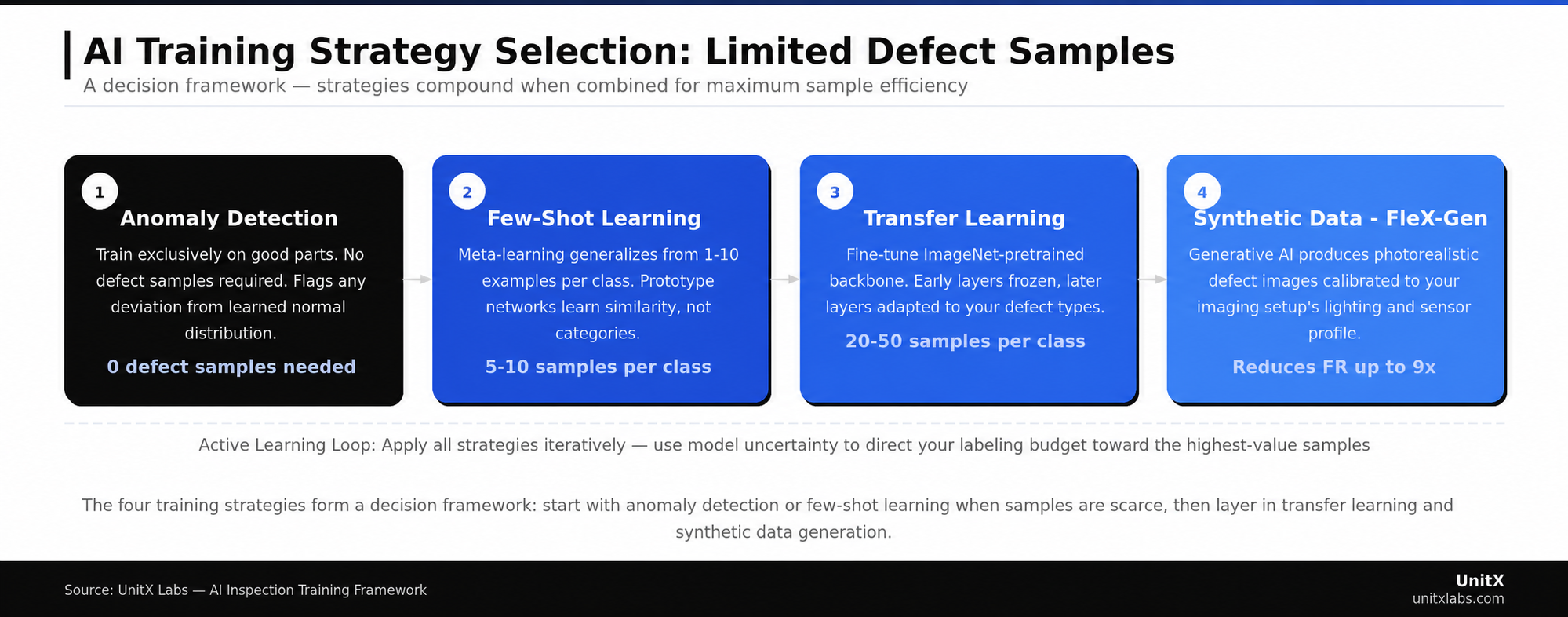
The four training strategies form a decision framework based on available sample count and defect type diversity. Each approach can be combined with the others for compounding gains.
3. Anomaly Detection: Eliminate the Defect Sample Requirement Entirely
For certain inspection scenarios, the most efficient path to a production model is to train exclusively on good parts. Anomaly detection methods learn a statistical model of what “normal” looks like, then flag any image that deviates sufficiently from that distribution as a potential defect. Because you only need normal samples for training — which are abundant on any production line — the labeled defect sample problem disappears.
Modern anomaly detection architectures using memory bank-based methods like PatchCore and flow-based models have reached near-supervised accuracy on standard benchmarks. The tradeoff is reduced specificity: the model can tell you that something is wrong, but not always which defect class is present. For applications where defect classification is secondary to zero-escape detection, this is often an acceptable tradeoff.
A practical limitation is that anomaly detection methods can struggle with normal parts that have high natural variability — for example, cast components with variable surface grain. In these cases, hybrid approaches that combine anomaly detection with a few-shot classifier for confirmed defect types deliver the best of both worlds.
4. Synthetic Data Generation: Engineer the Training Set You Need
When neither real samples nor anomaly detection are sufficient, generative AI can create the training data from scratch. GAN-based approaches and diffusion model methods have both demonstrated the ability to generate photorealistic synthetic defect images that improve real-world model performance when added to training sets.
Research on diffusion model-based defect generation for steel surfaces demonstrated that synthetic defect images generated under few-shot conditions contributed to measurable improvements in detection performance on real datasets. For EV battery and semiconductor inspection — where rare defect types can represent catastrophic failure modes — the ability to generate synthetic examples of edge-case defects is especially valuable. Learn how FleX-Gen applies generative AI to this exact problem.
The key constraint on synthetic data is physical fidelity. Generated images that do not faithfully reproduce the lighting, texture, and sensor characteristics of your actual inspection setup create a domain gap that degrades rather than improves model performance. Effective synthetic data generation requires careful calibration to your specific imaging conditions.
The Data Quality Multiplier: Why Imaging Setup Matters More Than Sample Count
The most common mistake in low-data AI training is treating sample count as the only variable. In practice, data quality is the dominant factor — and poor-quality data at high volume performs worse than high-quality data at low volume.
Imaging Consistency
A model trained on images captured under inconsistent lighting will fail when lighting conditions shift slightly on the production line. Defect visibility is highly lighting-dependent: certain scratch orientations are only visible under specific illumination angles, and subsurface porosity may only appear under darkfield or coaxial lighting. Before collecting defect samples, invest in a stable, repeatable imaging setup. Variable illumination is the single most common cause of model performance degradation in deployment that was not predicted during validation.
AI-powered imaging systems with software-defined illumination control — where independent lighting channels can be precisely configured and reproduced — eliminate this variable entirely. When the imaging setup is stable, every sample collected carries consistent information, maximizing the learning signal from each labeled image.
Labeling Consistency
In limited-sample scenarios, label noise has an outsized impact. If three quality engineers classify the same borderline scratch differently — two call it a defect, one passes it — your 30-sample dataset effectively contains 30 conflicting signals. Research consistently shows that inter-annotator disagreement on defect boundaries and severity thresholds is a primary source of training instability in industrial AI models.
Establish written labeling standards before collecting samples. Define what constitutes a defect versus an acceptable cosmetic variation with reference images. For ambiguous cases, implement a consensus protocol. Consistent labels from 20 samples outperform inconsistent labels from 200 samples. For more on this topic, explore the UnitX technical blog.
Data Augmentation: Expanding a Small Dataset Without Synthesis
Between collecting real samples and deploying generative AI, data augmentation occupies a practical middle ground. Standard augmentations — horizontal flipping, rotation, brightness and contrast perturbation, and Gaussian noise — effectively multiply your labeled dataset by presenting the same defect in varied forms. For surface defects that are directionally symmetric, these transforms are safe and reliable.
However, not all augmentations are appropriate for all defect types. Research on weld defect classification found that rotating weld images by 90 degrees actually reduced model accuracy because weld direction is semantically meaningful for that defect category. Domain knowledge about your specific defect type should govern augmentation strategy. Geometric transforms that change the orientation of directional defects may corrupt the label rather than enrich the training set.
More sophisticated augmentation techniques — mosaic augmentation, CutMix, and feature-space interpolation — have demonstrated additional gains on imbalanced industrial datasets. These methods are available in most modern training frameworks and can be applied with minimal engineering overhead. See how CorteX handles sample-efficient training in production environments.
Active Learning: Spend Your Labeling Budget Where It Counts
When you have a large pool of unlabeled images and a limited labeling budget, active learning helps you identify which unlabeled examples — if labeled — would provide the greatest improvement to your model. The model selects its own training examples based on uncertainty or expected information gain, rather than labeling images at random.
For defect detection, the practical workflow is: train an initial model on your small labeled set, run it on a large unlabeled pool, identify the images where the model is most uncertain, send those images to a labeler, retrain, and repeat. This loop concentrates your labeling effort on the examples that actually matter — boundary cases, rare defect orientations, and edge-case lighting conditions — rather than accumulating more examples of defect types the model already handles confidently.
A Framework for Choosing the Right Strategy
| Scenario | Recommended Strategy | Min. Samples Needed |
| Zero defect samples available | Anomaly detection (normal-only training) | 0 defect / ≥50 normal |
| 1–10 samples per defect class | Few-shot learning + augmentation | 5–10 per class |
| 10–50 samples per defect class | Transfer learning + augmentation | 20–50 per class |
| New defect type, no real examples | Synthetic data generation (FleX-Gen-type) | 0 real / synthetic generated |
| Large unlabeled pool, small labeled set | Active learning loop | ~20 initial labeled |
Validation: The Discipline That Makes Low-Data Models Trustworthy
With limited samples, the risk of overfitting to your training set is real. A model that achieves 99% accuracy on 30 training images may generalize poorly to production conditions. Rigorous validation discipline is what separates a reliable production model from a demo that fails at go-live.
Hold out a strict validation set — separate from the training data — that was not used in any training decision, including hyperparameter selection. For very small datasets, use k-fold cross-validation to obtain a stable performance estimate. Validate on images captured at different times, different shifts, and, if possible, under slightly varied lighting — not just on a clean set collected in a single session. Production conditions are never identical to controlled validation conditions, and your model should demonstrate robustness to those variations before deployment. Review the UnitX customer case studies for examples of how this validation framework applies across automotive and battery production lines.
Common Questions
How many defect samples do I actually need to start training?
With modern sample-efficient architectures, you can begin meaningful model development with as few as 5 images per defect category. This is sufficient for initial few-shot or anomaly-detection-based models that give you a performance baseline. A production-ready model — one deployed to a live line — typically requires 20–50 well-labeled samples per class when using transfer learning, though the exact number depends on defect complexity and imaging consistency.
Does synthetic data actually improve real-world inspection accuracy?
Yes, under specific conditions. Synthetic data is effective when it accurately replicates your imaging setup’s lighting, resolution, and sensor noise. Domain-mismatched synthetic images — generated from generic 3D renders that do not match your actual camera characteristics — can degrade model performance. The most effective synthetic data strategies involve generating images within the actual imaging pipeline rather than from external rendering tools.
What is the biggest mistake manufacturers make when training with limited data?
Inconsistent labeling is the most common and most damaging mistake. When quality engineers disagree on which images constitute defects — especially for borderline severity levels — the training set contains conflicting signals that a limited-sample model cannot resolve. Establishing a clear, documented labeling standard with reference examples before collecting any training data is the single highest-leverage action for improving model quality on small datasets.
Can I use the same model across multiple product variants?
Not without adaptation in most cases. Product variants with different geometries, surface finishes, or materials produce images that differ sufficiently from your original training set to degrade performance. Transfer learning helps here: fine-tune your existing model on a small set of samples from the new variant rather than retraining from scratch. This typically requires 10–30 new labeled samples per defect class.
How do I know when my model is ready for production deployment?
The threshold depends on your quality requirements. Define your target False Acceptance Rate (FA) and False Rejection Rate (FR) before training — for example, FA = 0% and FR ≤ 1%. Validate on a blind holdout set that the model has never seen. If the model meets your FA and FR targets on the holdout set across at least 500 total images (including normal parts), it is a candidate for supervised pilot deployment. Run the pilot alongside manual inspection before removing human oversight entirely.