Area Under the Curve AUC Machine Vision System Definition and Importance

June 16, 2025

SHARE ALSO

The area under the curve (AUC) machine vision system uses AUC as a powerful way to measure how well a binary classification model separates positive and negative classes. In machine vision, AUC evaluates the model’s ability to correctly identify objects or features in images. The ROC curve plots true positive rates against false positive rates, and the area under the curve shows the overall performance of the model. Experts use the AUC ROC curve to compare different models, especially in image classification and object detection. Studies show that AUC-ROC scores, such as those in DataCamp tutorials, demonstrate how close a model comes to perfect discrimination. In complex tasks like medical image analysis, researchers often extend ROC analysis with LROC or FROC curves to better capture the area under the curve (AUC) machine vision system performance. These approaches help ensure the model provides reliable results.

Key Takeaways

AUC measures how well a machine vision model separates positive and negative classes by summarizing its ability to rank images correctly.
The ROC curve plots true positive rates against false positive rates, and the area under this curve (AUC) shows overall model performance across all thresholds.
High AUC values indicate strong model accuracy and help compare different models in tasks like image classification and medical imaging.
AUC is robust to changes in class distribution and works well even with limited data, but it should be used alongside other metrics like precision and recall for a full evaluation.
While AUC offers a clear, single value for model discrimination, it may hide issues in imbalanced datasets and does not measure clinical usefulness or error costs.

AUC in Machine Vision Systems

What is AUC?

The area under the curve (AUC) machine vision system uses AUC as a key metric to evaluate how well a model separates positive and negative classes. In machine vision, AUC measures the probability that a model ranks a randomly chosen positive image higher than a randomly chosen negative one. This metric is closely linked to the ROC curve, which plots the true positive rate against the false positive rate at different thresholds. AUC provides a single value that summarizes the model’s ability to discriminate between classes, making it a popular choice in computer vision tasks.

Researchers often use AUC-ROC to compare models in image classification and object detection. For example, in medical imaging, high AUC values show that a model can accurately distinguish between healthy and diseased images. Studies have shown that AUC remains reliable even when data is limited, especially when using advanced cross-validation methods like leave-pair-out cross-validation. This approach reduces bias and variance in AUC estimates, making the area under the curve (AUC) machine vision system more dependable in real-world applications.

AUC scores range from 0 to 1. A score of 0.5 means the model performs no better than random guessing. Scores closer to 1 indicate strong discrimination between classes. A perfect score of 1 means the model always ranks positive images above negative ones. In contrast, a score below 0.5 suggests the model is making poor or inverted predictions.

Note: AUC is threshold-independent. This means it evaluates model performance across all possible thresholds, not just a single cutoff. This property makes AUC robust, especially when dealing with imbalanced datasets.

How AUC Works

AUC works by analyzing the ROC curve, which shows the trade-off between the true positive rate and the false positive rate as the decision threshold changes. The area under the ROC curve represents the model’s overall ability to distinguish between positive and negative classes. The ROC curve starts at the origin (0,0) and ends at the point (1,1). As the threshold lowers, both the true positive rate and false positive rate increase, creating a curve that moves toward the top-left corner for better models.

The AUC-ROC value is calculated using numerical integration methods, such as the trapezoidal rule. This process sums the area under the ROC curve, giving a single number that reflects model performance. Statistically, AUC represents the chance that the model will rank a positive instance higher than a negative one. This interpretation links the ROC curve’s geometric shape to a probabilistic ranking measure.

AUC-ROC is especially useful in machine vision because it does not depend on the class distribution. For example, in a study on disease classification, models achieved AUC values as high as 0.947 and even 1.000, showing excellent performance in distinguishing between different medical conditions. In another case, a fraud detection system improved its AUC from 0.75 to 0.88 after model tuning, leading to fewer false alarms and better accuracy.

The area under the curve (AUC) machine vision system also benefits from stability across different datasets. A large simulation study found that AUC had the smallest variance and most stable ranking among 18 metrics, making it a reliable choice for binary classification tasks. This stability holds even when the prevalence of positive and negative classes changes.

AUC-ROC works alongside other metrics, such as precision, recall, and F1 score, to provide a complete picture of model performance. The table below compares these metrics:

Metric	Purpose	Ideal Value	Importance in Model Evaluation
Precision	Correct positive predictions	High	Crucial when false positives are costly or minimizing false detections is important.
Recall	Identify all positive instances	High	Essential when missing positive cases is costly or detecting all positives is vital.
F1 Score	Balanced performance	High	Useful for imbalanced datasets or when false positives and false negatives have different costs.
AUC	Overall classification performance	High	Important for assessing model performance across thresholds and comparing different models comprehensively.

AUC-ROC also connects to the confusion matrix, which shows the counts of true positives, false positives, true negatives, and false negatives. While the confusion matrix gives detailed results at a specific threshold, AUC-ROC summarizes performance across all thresholds. This makes the area under the curve (AUC) machine vision system a valuable tool for model selection and evaluation.

AUC ROC Curve

ROC Curve Basics

The ROC curve, or receiver operating characteristic curve, is a fundamental tool in machine vision for evaluating binary classification models. This curve plots the true positive rate against the false positive rate at different thresholds. By adjusting the threshold, the model produces various combinations of these rates, which form the ROC curve. The area under this curve, known as AUC, measures how well the model separates positive and negative classes.

Researchers often use real-world datasets to illustrate ROC curve construction. For example, the Iris dataset helps demonstrate how a model, such as logistic regression, assigns scores to samples. By changing the threshold, the ROC curve shows the trade-off between sensitivity and specificity. Visualizations, like those created with turtle graphics, make the process easy to understand. The ROC curve provides a clear picture of model performance across all thresholds, not just one.

Statistical analysis supports the use of the ROC curve and AUC in machine vision. The AUC ROC curve offers a threshold-independent measure, considering all possible decision points. Studies across many datasets and metrics show that AUC has the smallest variance and remains stable even when class distributions change. This stability makes the AUC ROC curve a reliable choice for comparing models.

Interpreting AUC ROC

Interpreting the AUC value from the ROC curve helps users understand model quality. The AUC ROC curve summarizes the model’s ability to rank positive instances higher than negative ones. A value close to 1 means the model performs well, while a value near 0.5 suggests random guessing.

Quantitative methods make interpreting AUC ROC straightforward. Tools like scikit-learn provide functions to compute the ROC curve, AUC, and AUC-ROC scores. For multi-class tasks, strategies such as one-vs-rest and one-vs-one extend the ROC curve and AUC to more complex problems. Averaging methods, like micro-averaging and macro-averaging, help handle class imbalance and aggregate results.

The ROC curve and AUC ROC curve remain valuable in machine vision because they are scale-invariant and robust to changes in class distribution. However, users should remember that AUC-ROC does not reflect the cost of errors and may not always suit highly imbalanced datasets. Still, the AUC ROC curve provides a comprehensive view of model performance, making it essential for model evaluation and selection.

Area Under the Curve (AUC) Machine Vision System Applications

Model Comparison

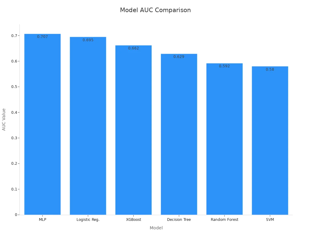
Researchers and engineers use auc and roc metrics to compare different machine vision models. These metrics help identify which model best separates positive and negative classes in tasks like image recognition and object detection. For accurate auc calculation, models must output prediction scores or probabilities, not just class labels. This approach allows the auc-roc curve to reflect the model’s ability to rank images correctly across all thresholds.

Academic studies provide clear examples of how auc guides model selection. In a comparative analysis of vision transformers and convolutional neural networks for diabetic retinopathy detection, the SWIN transformer achieved the highest auc values, such as 95.7% on the Kaggle test set. Other CNN models ranged from 86% to 94%. The study used statistical tests like DeLong’s test with Bonferroni correction to confirm that the differences in auc-roc scores were significant. Another publication compared CNN architectures for chest radiograph classification, showing that deeper models like ResNet-152 and DenseNet-161 reached auc-roc values around 0.88, outperforming shallower networks.

Note: To ensure fair comparison, researchers use statistical tests such as DeLong’s test to determine if differences in auc-roc scores between models are meaningful.

The table below shows how auc differences between models are tested:

Model Comparison	Model A AUC	Model B AUC	Statistical Test	Result Interpretation
Heart disease risk prediction	0.92	0.87	DeLong’s test, p < 0.05	Significant difference; Model A better
R implementation example	0.96	0.74	DeLong’s test, p = 0.09	Not statistically significant at 0.05 level

Practical Use Cases

The auc-roc metric plays a vital role in real-world machine vision applications. In medical imaging, models for cataract surgery phase recognition achieved auc values from 0.880 to 0.997, showing high accuracy and real-time usefulness. Deep learning models for keratitis screening reached aucs as high as 0.998, even when tested on smartphone images. Another study developed a system for papilledema detection, reporting aucs of 0.99 internally and 0.96 externally, proving strong generalizability across countries and ethnicities.

Industry reports highlight the impact of auc in laboratory automation and diagnostics. For example, a deep learning model reached an auc of 0.95 in distinguishing COVID-19 from other lung diseases. Automated lab systems reported mean aucs of 0.98 and 0.94 in various diagnostic tests, improving both speed and reliability.

Researchers use several metrics alongside auc-roc, such as the Kolmogorov-Smirnov score and Gini Index, to evaluate model performance. These metrics rely on predicted probabilities, not just labels, to assess how well a model ranks positive cases. Functions like roc_auc_score in Python’s sklearn library help calculate auc-roc using these probabilities. This method supports robust evaluation, especially when class imbalance or threshold selection matters.

AUC: Pros and Cons

Benefits

AUC offers several advantages for evaluating machine vision models. Many researchers prefer this metric because it provides a single, easy-to-understand value that summarizes how well a model separates positive and negative cases. AUC does not depend on a specific threshold, so it gives a complete view of model performance across all possible cutoffs. This property makes it especially useful when comparing models in tasks like disease diagnosis or object detection.

AUC balances sensitivity (true positive rate) and specificity (false positive rate), making it a comprehensive measure.
The metric remains robust even when class distributions change, which helps in real-world scenarios.
Studies show that AUC works well with complex models, such as those using two-parameter or three-parameter logistic structures.
AUC values range from 0.5 (random guessing) to 1 (perfect classification), so users can easily interpret results.
In practical applications, such as kidney disease detection, a high AUC (for example, 0.87) indicates strong model discrimination.
AUC is accessible and easy to compute using popular tools like Python, R, and MATLAB.

AUC also helps consolidate model discrimination into a single value, which supports efficient model ranking and selection. When combined with other metrics, AUC provides a holistic view of model effectiveness.

Limitations

Despite its strengths, AUC has important limitations. It mainly measures discrimination, not calibration or clinical usefulness. This means AUC may not reflect how well a model predicts actual risk or how useful it is in practice.

AUC can hide poor generalization, especially in imbalanced datasets. For example, a model might show a high AUC but perform poorly for minority classes, as seen in studies using the MIMIC-III dataset.
The metric is less sensitive to false positives in imbalanced data. Precision-recall curves often provide a clearer picture in these cases.
AUC does not capture all aspects of model performance, such as precision or negative predictive value. Users need to consider other metrics for a complete evaluation.
In some clinical settings, AUC may give an overly optimistic view of model performance, especially when the minority class is small.
Empirical studies show that AUC can mask deficiencies in detecting rare events, so relying only on AUC may lead to misleading conclusions.

Tip: Always use AUC alongside other metrics, such as precision, recall, and F1 score, to ensure a thorough assessment of model performance.

AUC stands as a key measure for evaluating machine vision systems. High AUC values, such as 0.92 for patient-level diagnostics, show strong model accuracy and reliability. Meta-analyses confirm that AUC and AUC-ROC help compare models and support robust selection.

Proper study design and statistical methods ensure valid AUC results.
Combining AUC with sensitivity, specificity, and F1 score gives a complete view.

AUC works best when used with other metrics for balanced model evaluation.

FAQ

What does the ROC curve show in machine vision?

The ROC curve shows how well a model separates positive and negative classes. It plots the true positive rate against the false positive rate. This curve helps engineers see the trade-off between sensitivity and specificity for different thresholds.

How does the confusion matrix relate to model performance?

The confusion matrix displays the number of correct and incorrect predictions for each class. It helps users understand model performance by showing true positives, false positives, true negatives, and false negatives. This table gives a detailed view at a specific threshold.

Why is a high AUC important in binary classification models?

A high AUC means the model can distinguish between positive and negative cases very well. This value shows strong discrimination ability. In binary classification models, a high AUC often leads to better decision-making in real-world tasks.

What is the receiver operating characteristic curve?

The receiver operating characteristic curve, or ROC curve, is a graph that shows the performance of a classification model at all thresholds. It helps users compare different models and choose the best one for their needs.

How do experts approach interpreting the AUC value?

Experts look at the AUC value to judge how well a model ranks positive cases above negative ones. A value close to 1 means excellent performance. A value near 0.5 suggests the model does not perform better than random guessing.