There’s a specific kind of frustration that QA engineers know well: your inspection system catches a cosmetic scratch that doesn’t affect product function, rejects the part, a line operator overrides it, and the override gets logged as an “exception.” Do this a thousand times and you’ve built a quality control process that relies on human judgment to compensate for a system that’s too sensitive in the wrong places and not sensitive enough in the right ones.
The root cause, in most cases, is how the underlying AI model represents what it sees. And the most important distinction isn’t between AI and non-AI — it’s between systems that use bounding boxes to locate defects and systems that use semantic segmentation to understand them at the pixel level.
Key Takeaways
- Semantic segmentation classifies every pixel in an image, not just a rectangular region — giving you the exact size, shape, and location of each defect.
- Bounding box detection creates coarse approximations that force conservative acceptance thresholds, leading to high false rejection rates on variable surfaces.
- Pixel-level output enables zone-based rejection logic: the same defect type can be acceptable in one area of a part and rejectable in another, matching real QA criteria.
- Semantic segmentation is computationally intensive but modern edge hardware handles it at production line speeds — UnitX CorteX processes at up to 100 MP/s.
Segmentation vs. Detection: An Analogy That Actually Explains It
The Bounding Box Approach
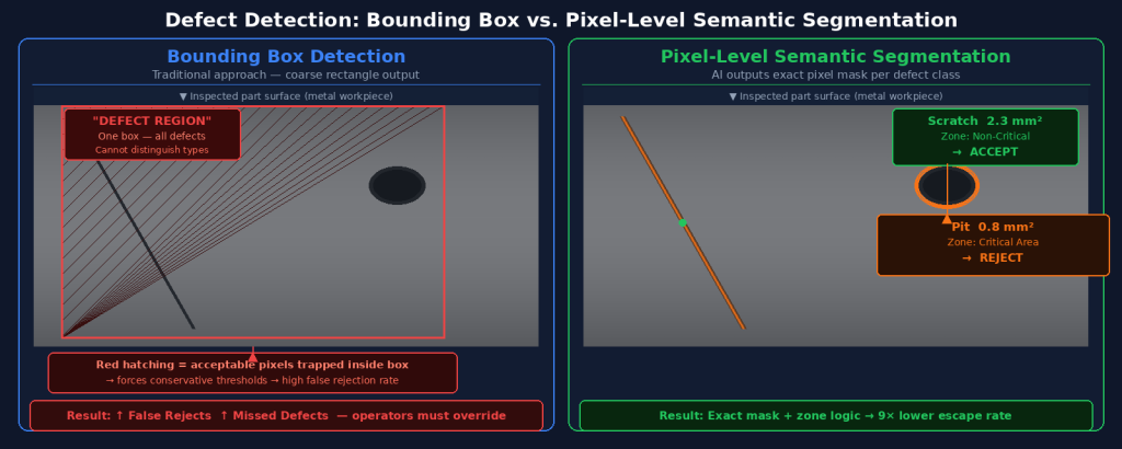
Imagine asking someone to describe the damage on a car door by drawing rectangles around damaged areas. Even if the rectangles are accurate, you lose critical information: exactly which pixels are damaged, how large the actual damage is, whether it extends to an edge or stops before a functional surface. The rectangle tells you where to look but not what exactly is there.
Bounding box object detection works the same way in machine vision. The model identifies a region of interest and assigns it a class label (“scratch,” “dent,” “contamination”) but provides only a coarse approximation of the defect’s extent. For acceptance logic purposes, this means you must make worst-case assumptions: treat the entire bounding box as defective, even if only 15% of its pixels actually are.
What Semantic Segmentation Does Instead
Semantic segmentation assigns a class label to every individual pixel in the image. For defect detection, this means the model outputs a precise mask: these 342 pixels are a scratch, these 89 pixels are a contamination point, and these remaining 1.2 million pixels are acceptable surface. The output is not an approximation — it is the actual defect, at full resolution.
This pixel-level precision changes what’s possible in downstream acceptance logic. You know the exact area of the defect in mm² (once calibrated to physical dimensions). You know whether it crosses a critical zone. You know its aspect ratio, which can distinguish a processing mark from a structural crack. And you can set acceptance criteria that match how your quality engineers actually think about defects — not “is there anything suspicious here?” but “is there a defect of this type, in this location, of this size?”
The Technical Architecture Behind Semantic Segmentation
Encoder-Decoder Networks
Modern semantic segmentation models use an encoder-decoder architecture. The encoder (typically a pre-trained backbone like ResNet or EfficientNet) processes the input image through successive convolutional layers, progressively reducing spatial resolution while extracting rich feature representations. The decoder then reconstructs spatial resolution through upsampling operations, using the encoded features to produce a full-resolution output map where each pixel has a class probability.
The key innovation in architectures like U-Net — widely used in industrial segmentation — is the use of skip connections between encoder and decoder layers. These connections preserve fine-grained spatial detail that would otherwise be lost during the encoder’s downsampling, which is critical for detecting small defects (sub-millimeter scratches, micro-porosity) that might occupy only a few dozen pixels in a high-resolution image.
Handling Class Imbalance: The Defect Detection Challenge
One of the practical challenges in training segmentation models for defect detection is class imbalance. In most production environments, defective pixels represent a tiny fraction of total image pixels — often less than 0.1%. Standard cross-entropy loss functions treat every pixel equally, which means a model can achieve 99.9% pixel accuracy by simply predicting “normal” for everything, never detecting a single defect.
Addressing this requires specialized loss functions (weighted cross-entropy, Focal loss, Dice loss) that up-weight the contribution of defect pixels during training. Research published in Scientific Reports (2024) demonstrated that semi-supervised segmentation approaches with proper class-balancing techniques achieved mean IoU (Intersection over Union) improvements of 3–4% over baseline methods on industrial defect datasets — a meaningful gain when your acceptance spec requires catching every scratch over 0.5mm.
Why Pixel-Level Output Matters for QA Logic
Zone-Based Acceptance Criteria
One of the most powerful capabilities enabled by pixel-level segmentation is zone-aware inspection. Most manufactured parts have areas where defects are critical and areas where they are cosmetically acceptable. A scratch on the sealing surface of an O-ring groove is a functional failure. The same scratch on the chamfer of a non-functional edge is a cosmetic mark that experienced inspectors would accept.
Bounding box systems cannot implement this logic reliably because their spatial resolution is insufficient to determine which zone a defect occupies. Pixel-level segmentation can, because the exact boundary of the defect is known. The acceptance engine can then evaluate: does any pixel of this defect mask overlap with the defined critical zone? If yes — reject. If no — accept, even if the defect is visually obvious.
Quantitative Defect Characterization
Beyond zone logic, pixel-level output enables defect characterization that adds engineering insight rather than just pass/fail decisions. For each detected defect, you can output: area in mm², maximum linear dimension, orientation angle, distance from nearest critical feature, and defect class with confidence score. This data supports downstream analysis — trend detection, process capability studies, supplier quality reports — that bounding box systems simply cannot provide with the same fidelity.
| Defect Output Parameter | Bounding Box Detection | Semantic Segmentation |
|---|---|---|
| Exact defect area (mm²) | ❌ Approximated by box area | ✅ Calculated from pixel mask |
| Defect location within part | ❌ Box center only | ✅ Exact boundary coordinates |
| Zone-based acceptance logic | ❌ Not reliably possible | ✅ Pixel-precise zone overlap check |
| Defect shape classification | ❌ Lost in box approximation | ✅ Aspect ratio, elongation, curvature |
| False Rejection control | ❌ Conservative thresholds required | ✅ Precise per-class, per-zone thresholds |
Semantic Segmentation at Production Line Speeds
The Computational Reality
Semantic segmentation is computationally heavier than bounding box detection. A U-Net inference pass on a 2048×2048 image requires significantly more computation than running a YOLO detector on the same image. For years, this made segmentation impractical for high-speed production lines. Modern edge GPU hardware has changed this calculus.
UnitX CorteX Inference runs at up to 100 megapixels per second, enabling segmentation-quality inspection at throughputs of up to 1,200 parts per minute — covering the majority of high-volume manufacturing applications. The inference runs on edge hardware co-located with the imaging station, with no dependency on cloud connectivity or central server availability, which is critical for environments where network latency or connectivity is unreliable.
Hardware-Software Co-Design
One reason UnitX achieves these inference speeds is that the imaging and AI layers are designed together. The OptiX imaging system is engineered to produce images that match the input characteristics the CorteX segmentation models were trained on — consistent resolution, calibrated illumination, predictable noise characteristics. This hardware-software co-design avoids the degradation that occurs when AI models trained in one imaging environment are deployed against images from a different camera or lighting setup.
Practical Implications for QA Teams
If you’re evaluating AI inspection platforms, the segmentation vs. bounding box distinction should be a first-order question in your evaluation. Ask specifically: does this system output pixel-level masks, or bounding boxes with class labels? What does the acceptance logic engine look like — can you define zone-based criteria, or only global thresholds?
For production environments where surface variation is high (machined metals, cast parts, coated surfaces), where defect types have different criticality depending on location, or where False Rejection rates above 2% create downstream labor costs — semantic segmentation is not a premium feature. It is the baseline requirement for a system that can actually match the nuance of your quality standards.
→ See how CorteX’s pixel-level segmentation enables precise threshold control and zone-based acceptance logic across UnitX deployments.
Frequently Asked Questions
Is semantic segmentation the same as instance segmentation?
No. Semantic segmentation assigns a class to every pixel, but treats all pixels of the same class as belonging to the same category — so two overlapping scratches would be labeled as the same “scratch” region. Instance segmentation goes further by distinguishing individual instances — each scratch would be labeled as a separate object. For most defect detection applications, semantic segmentation is sufficient; instance segmentation becomes relevant when you need to count discrete objects (missing fasteners, distinct foreign particles) rather than classify surface conditions.
Can semantic segmentation models be trained with small datasets?
Traditional segmentation architectures (fully supervised training from scratch) require thousands of labeled examples to generalize well. Few-shot and semi-supervised approaches can work with significantly fewer labels. In practice, the most effective approach for production deployments combines a small set of real defect annotations with synthetic defect data generation — using tools like UnitX GenX — to produce training sets large enough for robust models without requiring months of data collection from the production line.
How does 2.5D imaging interact with semantic segmentation?
2.5D imaging adds a depth channel to the standard RGB or grayscale image, providing per-pixel height information. When input to a semantic segmentation model, this depth channel provides geometric cues — actual surface topology — that 2D models cannot access. This is especially valuable for distinguishing visually similar features that differ in their geometric profile: a polishing mark and a grinding burr may look nearly identical in 2D, but their depth signatures are distinct. UnitX OptiX’s 2.5D capability feeds this geometric information directly into CorteX’s segmentation pipeline.