Every pixel delivered by an industrial camera is contaminated — to some degree — by sensor noise, optical aberrations, motion blur, or environmental interference. Image filtering is the set of mathematical operations used to separate the signal you want from the noise you do not. Understanding the available filters, what each one does to the image, and when to apply each type is one of the most practical skills in machine vision system design. This guide covers the filters used in real industrial inspection pipelines, with enough technical grounding to make principled choices.
Key Takeaways
- Image filtering applies a convolution kernel — a small matrix of weights — to each pixel neighborhood, transforming the image to enhance or suppress specific spatial frequency content.
- Smoothing filters (Gaussian, median, bilateral) reduce noise; sharpening filters (Laplacian, unsharp mask) enhance edge contrast; edge detection filters (Sobel, Canny) isolate boundaries.
- The bilateral filter is the only classical smoothing filter that simultaneously reduces noise and preserves edges — making it the preferred choice when feature boundaries must remain intact during preprocessing.
- Choosing the wrong filter — for example, applying Gaussian smoothing before edge-based defect detection — can degrade both algorithm performance and inspection accuracy.
What Is Image Filtering and How Does Convolution Work?
The Convolution Operation
Image filtering is implemented through convolution: sliding a small matrix called a kernel (or filter) across every pixel in the image, computing a weighted sum of the pixel and its neighbors at each position, and writing the result to the output image. The kernel encodes the operation to be performed — its specific pattern of weights determines whether the output will be blurred, sharpened, edge-enhanced, or noise-reduced.
Mathematically, for a 2D image I and kernel K, the output at pixel (x, y) is:
Output(x,y) = sum over i,j of: K(i,j) × I(x+i, y+j)
As described in the Wikipedia kernel reference: “The values of a given pixel in the output image are calculated by multiplying each kernel value by the corresponding input image pixel value, and summing up the results.” A 3×3 kernel size is most common in practice, as it captures immediate neighborhood context while remaining computationally efficient.
Spatial Noise: What Filters Are Trying to Remove
Spatial noise in machine vision images originates primarily from camera sensor imperfections: variations in individual pixel sensitivity (fixed-pattern noise), random thermal electron emission (dark current noise), and photon arrival randomness (shot noise). Environmental sources — such as EMI from nearby motors, vibration-induced focus shift, and thermal gradients across the sensor — also contribute.
As documented in Edge AI Vision’s analysis of spatial noise reduction: “Spatial noise in imaging is the variation or irregularity in pixel values that is unrelated to the actual features of the scene being captured.” This type of noise occurs at the pixel level and can introduce unwanted artifacts. Understanding the type of noise present in your system drives filter selection more than any other factor.
Smoothing Filters: Reducing Noise
Box (Average) Filter: Fast but Crude
The simplest smoothing filter replaces each pixel with the arithmetic mean of its neighborhood. The kernel is a matrix of equal weights. A 3×3 box filter kernel looks like:
1/9 × [ 1 1 1 ]
[ 1 1 1 ]
[ 1 1 1 ]
The box filter reduces random noise through averaging, but it severely blurs edges and introduces ringing artifacts at sharp transitions. It has limited use in precision inspection systems, but can be useful for rapid preview filtering or in cases where sharpness is irrelevant (e.g., background suppression).
Gaussian Filter: The Standard Noise Smoother
The Gaussian filter weights neighbors pixels according to a bell-curve (Gaussian) function based on their distance from the center pixel. Nearby pixels contribute more than distant ones, producing a smoother blur than the box filter and significantly fewer ringing artifacts. A 3×3 approximation:
1/16 × [ 1 2 1 ]
[ 2 4 2 ]
[ 1 2 1 ]
Gaussian filtering is the industry standard for reducing Gaussian noise (the most common type of sensor noise) before subsequent processing steps. The kernel size (sigma parameter) controls the tradeoff: a larger sigma removes more noise but also blurs finer details. A key advantage of Gaussian filters is that they are separable — a 2D Gaussian can be applied as two successive 1D passes, significantly reducing computation for large kernels.
Median Filter: Salt-and-Pepper Noise Specialist
The median filter replaces each pixel with the median (not the mean) of its neighborhood values. Because the median is robust to extreme outliers, it is uniquely effective against salt-and-pepper noise — isolated bright or dark pixels caused by dead sensor pixels, cosmic ray events, or electrical interference — while preserving edge sharpness better than the box or Gaussian filters.
Research published in Scientific Reports (March 2025) on hybrid denoising algorithms confirms this distinction: “Median filtering is not effective for Gaussian noise. Therefore, a combination of adaptive median filtering and weighted median filtering was used to enhance the performance” in Gaussian noise scenarios.
The median filter’s ability to preserve edge makes it valuable in inspection systems where defect boundaries must remain clearly defined after noise reduction.
Bilateral Filter: Edge-Preserving Smoothing
The bilateral filter is the most sophisticated of the classical smoothing filters. It computes a weighted average of neighboring pixels using two factors simultaneously: (1) spatial proximity (like Gaussian filtering) and (2) intensity similarity. Pixels that are close in space and similar in intensity are given high weight, while pixels across an edge (with different intensities) are assigned near-zero weight, even if they are spatially close.
The result is smoothing that suppresses noise within homogeneous regions while preserving sharp edges. This makes the bilateral filter ideal for inspection preprocessing when both noise reduction and edge preservation are required. The tradeoff is computational cost — bilateral filtering is significantly slower than Gaussian filtering for equivalent kernel sizes, although GPU acceleration largely mitigates this limitation in modern vision systems.
| Filter | Noise Type | Edge Preservation | Speed |
| Box (Average) | All (weakly) | Poor | Fastest |
| Gaussian | Gaussian noise | Moderate | Fast (separable) |
| Median | Salt-and-pepper | Good | Moderate |
| Bilateral | Gaussian + preserves edges | Excellent | Slower |
Edge Detection Filters: Locating Defect Boundaries
Sobel Filter: Gradient-Based Edge Detection
The Sobel filter computes the image gradient — the rate of change of intensity — in the horizontal (Gx) and vertical (Gy) directions simultaneously using two convolution kernels:
Gx = [ -1 0 +1 ] Gy = [ -1 -2 -1 ]
[ -2 0 +2 ] [ 0 0 0 ]
[ -1 0 +1 ] [ +1 +2 +1 ]
Gradient magnitude = Gx2+Gy2 . A high gradient magnitude indicates an edge. The Sobel operator is weighted to give greater influence to the immediate neighbors of the current pixel (the center row/column values of 2), providing a degree of smoothing alongside edge detection.
As described in GeeksforGeeks’ convolution kernels reference, edges detected using Sobel “are sharper in comparison to Prewitt filters” due to this emphasis on immediate neighbors. Sobel is the workhorse edge detector in rule-based machine vision systems for tasks such as identifying component boundaries on a PCB, locating thread profiles on fasteners, or measuring gap dimensions.
Canny Edge Detector: The Multi-Stage Standard
The Canny edge detector is not a single convolution kernel but a four-stage algorithm: (1) Gaussian smoothing to suppress noise, (2) gradient computation (typically using Sobel), (3) non-maximum suppression to thin wide edge regions into single-pixel lines, and (4) hysteresis thresholding to trace connected edge chains while rejecting isolated noise responses.
The result is clean, single-pixel-wide edge maps that are significantly more useful than raw Sobel output for measurement tasks. Canny is the standard choice when edge localization accuracy — rather than just edge presence — is required.
Laplacian Filter: Second-Derivative Edge Detection
While Sobel computes first-order gradients (rate of change), the Laplacian computes the second derivative — identifying where the gradient itself is changing most rapidly. Zero crossings in the Laplacian correspond to edge locations. The Laplacian is rotationally symmetric (responding equally to edges in all directions), unlike Sobel. However, it is more sensitive to noise, which is why it is almost always applied after Gaussian smoothing (the “Laplacian of Gaussian” or LoG operator).
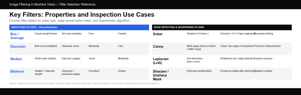
Key image filters in machine vision — grouped by purpose (noise reduction vs. edge detection vs. sharpening), each with different noise affinities and edge preservation characteristics.
Sharpening Filters: Enhancing Feature Contrast
Sharpening Kernel: High-Frequency Enhancement
The standard sharpening kernel amplifies the difference between a pixel and its neighbors, increasing local contrast and making edges appear crisper:
Sharpen = [ 0 -1 0 ]
[ -1 5 -1 ]
[ 0 -1 0 ]
The center coefficient (5) amplifies the pixel itself, while the negative surrounding values subtract the neighborhood average. This enhances fine texture and edge contrast but also amplifies noise — which is why sharpening filters should only be applied to pre-smoothed images when noise is present.
Unsharp Masking: Controlled Sharpening
Unsharp masking is a more controllable sharpening approach: a blurred (Gaussian-smoothed) version of the image is subtracted from the original, and a scaled version of that difference is added back. The operator parameters (amount and radius) allow precise control over which spatial frequencies are enhanced. Unsharp masking is the preferred sharpening method in production inspection systems where consistent, tunable enhancement is required.
From Classical Filters to Deep Learning: What Changed
Learned Convolutional Kernels in CNNs
The practical implication is significant: for a deep learning inspection model, preprocessing with classical filters is often redundant or even harmful. If the model is trained on raw sensor images, it learns to handle that sensor’s noise distribution directly. Applying a Gaussian blur before feeding images into a trained CNN effectively changes the input distribution the model was trained on — and typically degrades performance.
When Classical Filters Still Matter
Classical filters remain essential in three contexts in modern AI inspection systems:
- Rule-based preprocessing before feature extraction — When using classical algorithms (Hough circles, contour detection, thresholding) before neural network processing, filtering is often required to produce stable inputs.
- Data augmentation during training — Adding noise or blur to training images is a classical, filter-based augmentation strategy that improves model robustness to sensor variation.
- Post-processing depth maps and point clouds — Bilateral filtering is widely used to smooth noisy depth maps from stereo or structured light systems before dimensional measurement, since its edge-preserving properties prevent blurring of at object boundaries.
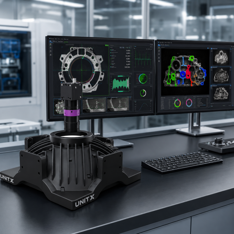
In UnitX’s CorteX system, the deep learning inference engine processes images from the OptiX multi-angle imaging front end without a classical preprocessing stage. The model is trained directly on the hardware’s native output, allowing it to learn the sensor’s specific noise characteristics and illumination patterns rather than working against them. For teams building inspection systems from scratch, understanding the interaction between preprocessing choices and model training is fundamental. The UnitX technical blog covers imaging and AI system design considerations for inline inspection in depth.
Practical Filter Selection Guide for Inspection Systems
Matching Filter to Application
The selection decision tree is driven by the downstream algorithm that consumes the filtered image and the type of noise present in the raw image:
- Passing images to a CNN inference model → Apply minimal or no preprocessing. Let the model handle the raw sensor output it was trained on.
- Passing images to threshold-based segmentation → Apply a Gaussian or bilateral filter first to stabilize threshold response. Use bilateral if boundary preservation matters; use Gaussian if speed is the priority.
- Passing images to edge-based measurement → Apply Gaussian smoothing, then Canny or Sobel. Never apply sharpening before edge detection — it amplifies noise responses.
- Sensor with dead pixels or ESD noise events → Use a median filter. No other filter removes salt-and-pepper noise as effectively.
- High-texture surfaces requiring fine-feature detection → Apply unsharp masking after Gaussian denoising to enhance feature contrast without introducing new noise.
For production inspection environments — particularly AI-powered systems performing inline surface defect detection — the interaction between imaging hardware, lighting design, and preprocessing choices is tightly coupled. Systems like UnitX CorteX make 100 MP/s AI inference practical precisely because the hardware front end (OptiX, with 32 independently controlled light channels) is designed to deliver clean, consistent images that minimize the preprocessing burden on the inference pipeline.
Frequently Asked Questions
What is the difference between a linear and a nonlinear filter?
Linear filters (box blur, Gaussian, Sobel, Laplacian, sharpening) operate by computing a fixed weighted sum of pixel values — the output is a linear combination of inputs. Nonlinear filters (median, bilateral) apply operations that cannot be expressed as simple weighted sums: the median selects a rank-order statistic, while the bilateral filter uses intensity-dependent weights that change with each pixel. Nonlinear filters are generally more effective at preserving edges and removing impulsive noise, but they are more computationally expensive and less easily GPU-parallelized than linear filters.
Why does the Gaussian filter blur edges?
Because it is a linear average of all neighbors within the kernel radius, weighted only by spatial distance — not by intensity similarity. Pixels on both sides of an edge contribute to the output, regardless of how different their intensities are. The larger the Gaussian sigma, the wider the blending zone around each edge. The bilateral filter addresses this limitation by incorporating intensity similarity, so only pixels with similar values (on the same side of the edge) contribute to the smoothing.
What is the relationship between image filtering and CNN feature maps?
Each channel in a CNN’s feature map is produced by convolving the input with a learned kernel — the same fundamental operation used in classical image filtering. The difference is that classical filter kernels are manually designed with specific spatial patterns, while CNN kernels are learned from data to detect task-relevant features. In early layers of a trained CNN, learned kernels often resemble classical filters (e.g., Gabor filters or edge detectors) because these represent the statistically optimal features in natural images. In deeper layers, they become increasingly abstract and task-specific.
Can I apply multiple filters in sequence?
Yes — sequential filter application is standard practice. The Canny edge detector, for example, is itself a three-filter sequence (Gaussian + gradient + non-maximum suppression). The Laplacian of Gaussian (LoG) combines Gaussian smoothing with second-derivative edge detection. Unsharp masking subtracts a blurred version of the image from the original. When sequencing filters, order matters: always denoise (smooth) before applying sharpening or edge detection, since sharpening amplifies all spatial frequency content — including noise.
How do I choose the kernel size for Gaussian filtering in an inspection system?
Kernel size determines how much of the surrounding neighborhood influences each output pixel. Larger kernels smooth over wider areas — effective for larger-scale noise, but increasingly destructive to fine features. A practical rule is to choose the smallest kernel that suppresses the dominant noise to acceptable levels, based on downstream algorithm performance (not just visual appearance). For typical CMOS sensors in industrial cameras, a 3×3 to 5×5 Gaussian kernel is usually sufficient. For large sensors or long-exposure captures with significant thermal noise, 7×7 to 9×9 may be needed. Always validate by measuring detection recall and precision on known defect samples after changing kernel size.