Why Gradient Descent Matters in Machine Vision Technology

July 5, 2025

SHARE ALSO

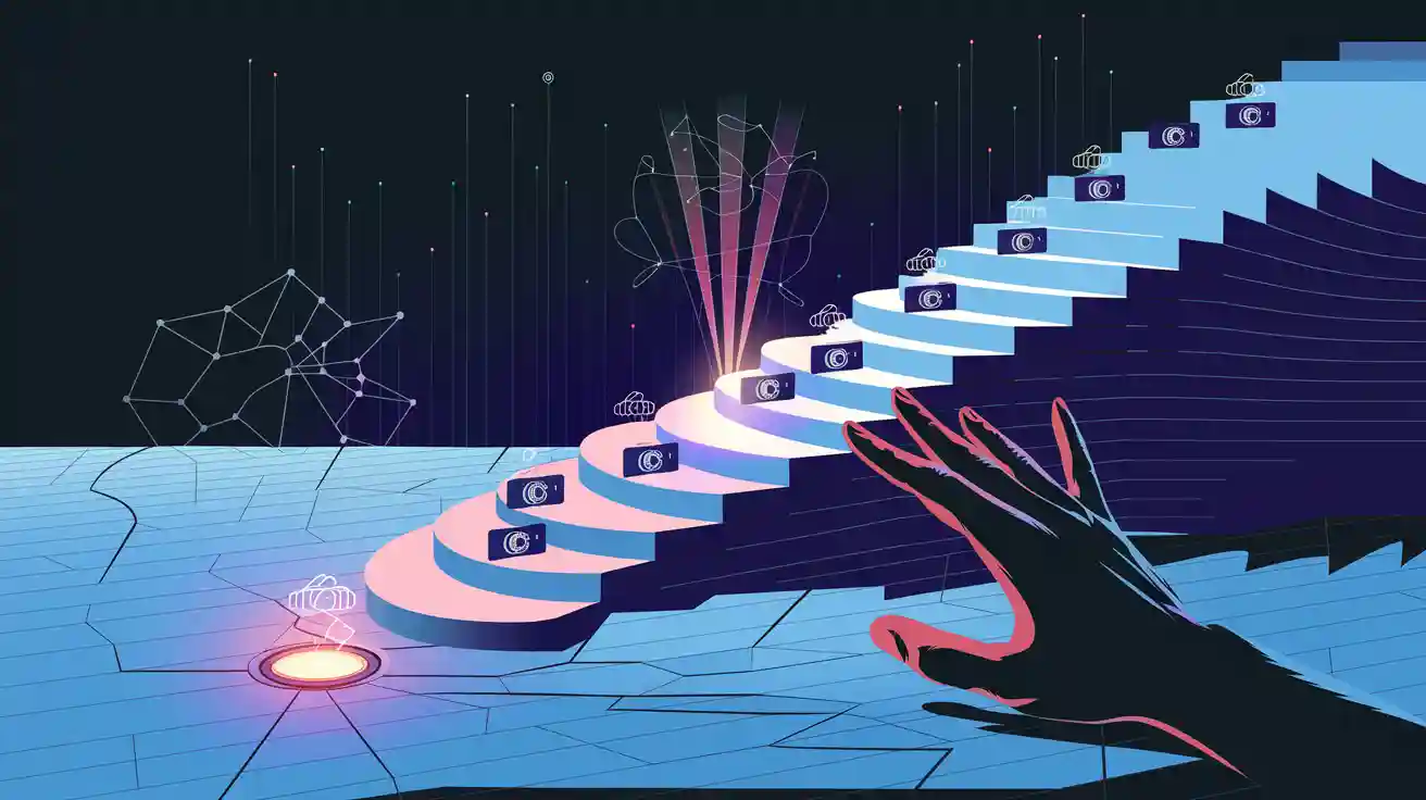
Gradient descent drives progress in machine vision systems by helping models learn from data and make better decisions. Leading companies like Tesla and Waymo use gradient descent machine vision system techniques to improve object detection, allowing cars to recognize pedestrians, vehicles, and traffic signs with high accuracy. This process involves updating model parameters to reduce mistakes, which is essential for safety and reliability. In these machine vision systems, object detection improves when gradient descent finds the best settings. Researchers note that tuning factors like learning rate and batch size in gradient descent machine vision system training leads to better performance, with strong statistical support for these improvements.

Machine vision systems depend on gradient descent for object detection and other key tasks, ensuring models remain accurate and adaptable.

Key Takeaways

Gradient descent helps machine vision systems learn by reducing errors step by step, improving accuracy in tasks like object detection and facial recognition.
Different types of gradient descent—batch, stochastic, and mini-batch—offer trade-offs between speed, stability, and memory use, with mini-batch often preferred for large datasets.
Tuning key factors like learning rate and batch size is crucial to avoid problems like local minima and unstable training, leading to better model performance.
First-order methods like stochastic gradient descent and momentum speed up learning and help models handle large, complex image data efficiently.
Continuous use of gradient descent allows machine vision systems to improve over time, adapting to new data and real-world challenges for reliable results.

Gradient Descent in Machine Vision Systems

Model Optimization

Machine vision systems rely on gradient descent to improve how they see and understand the world. When a gradient descent machine vision system learns, it adjusts its internal settings to make better predictions. This process is called model optimization. The system looks at the difference between what it predicts and what actually happens. It then changes its settings to reduce this difference.

Imagine a skier standing at the top of a mountain. The skier wants to reach the lowest point in the valley. Each step down the slope brings the skier closer to the bottom. In the same way, gradient descent helps machine vision systems move step by step toward the best settings. The system checks the slope, or gradient, of the error and takes a small step in the direction that reduces the error. Over time, these steps help the system find the lowest point, where the error is smallest.

Researchers have found that gradient descent works well for training machine vision models. Stochastic gradient descent, a popular version, handles noisy data and large images with many details. Deep learning models like ResNet, VGGNet, and YOLO use gradient descent with special tricks like momentum and learning rate schedules. These tricks help the models learn faster and more accurately. For example, the YOLOv6 model uses advanced gradient descent techniques to improve how it finds objects in pictures. Gradient descent also helps models avoid getting stuck in bad spots, called local minima, and works well with huge datasets, such as those used in facial recognition or self-driving cars.

Some common optimization techniques in machine vision systems include:

Learning rate scheduling, which changes how big each step is during training.
Momentum-based updates, which help the system move faster and avoid getting stuck.
Batch normalization, which keeps the system stable as it learns.
Weight decay, which stops the system from overfitting to the training data.
Adaptive learning rates, which adjust how quickly the system learns based on past steps.

These methods help the gradient descent machine vision system reach the best settings more quickly and accurately.

Cost Function Minimization

The heart of gradient descent in machine vision systems is the cost function. This function measures how far off the system’s predictions are from the real answers. The goal is to make this cost as small as possible. The cost function and loss function often mean the same thing in this context. They both show how well the system is doing.

For example, the cost function might use Mean Squared Error (MSE) or Mean Absolute Error (MAE). MSE punishes big mistakes more than small ones, while MAE treats all mistakes the same. By looking at the cost, the system knows how much it needs to improve. Each time the system makes a prediction, it checks the cost. If the cost is high, the system changes its settings to lower it. This process repeats many times, with the system always trying to make the cost smaller.

In a real-world example, a machine vision system might need to tell the difference between cats and dogs in photos. The cost function measures how many times the system gets it wrong. By minimizing errors, the system learns to make better choices. The process of minimizing the cost function guides the system to the best possible settings.

The cost function averages the mistakes over all the training data. This average, called empirical risk, helps the system learn from its errors. When the system minimizes the cost, it not only gets better at the training data but also improves on new, unseen data. For example, in predicting house prices, minimizing the MSE cost function helps the system avoid big mistakes and become more accurate.

Gradient descent makes this process possible. It helps machine vision systems find the best settings by following the slope of the cost function. This approach leads to smarter, more reliable systems that can handle real-world tasks like object detection, facial recognition, and more.

Tip: By focusing on cost function minimization, machine vision systems become more accurate and dependable in their predictions.

How Gradient Descent Works

Iterative Updates

Gradient descent helps machine vision models learn by making small changes to their settings over time. The process starts with the model making a guess. It then checks how far off this guess is by using a cost function. The cost function measures the difference between the model’s prediction and the real answer. If the difference is large, the model knows it needs to improve.

The model uses the slope, or gradient, of the cost function to decide which way to change its settings. This slope shows the direction that will reduce mistakes the fastest. The model takes a small step in that direction. This step is called an update. After each update, the model checks the cost function again. If the cost is still high, the model keeps updating its settings. This process repeats many times. Each step brings the model closer to the best answer.

Machine vision systems use this step-by-step approach to get better at tasks like object detection and image classification. The updates happen over many rounds, or iterations. With each round, the model learns from its errors and improves its predictions. The learning rate controls how big each step is. If the rate is too high, the model might miss the best answer. If the rate is too low, learning takes too long. Finding the right rate helps the model learn quickly and accurately.

Tip: Iterative updates allow machine vision models to learn from their mistakes and improve over time, making them more reliable in real-world tasks.

First-Order Methods

First-order methods use the gradient, or first derivative, of the cost function to guide updates. These methods look at how the cost function changes and use that information to make smart adjustments. Gradient descent is the most common first-order method. It helps models find the best settings by following the path of steepest descent on the cost function.

Stochastic gradient descent is a popular version used in machine vision. It updates the model using small batches of data, which makes learning faster and uses less memory. Stochastic gradient descent works well for large datasets and complex images. Researchers have found that using momentum with stochastic gradient descent helps the model move faster and avoid getting stuck. Momentum adds a "push" to each update, smoothing out the path and speeding up learning.

A modified Adam algorithm paper provides mathematical proofs showing improved convergence speed and accuracy compared to other optimizers.
Extensive experiments on two datasets show the modified Adam algorithm outperforms others in convergence speed and accuracy.
First-order methods use the gradient of the loss function to guide parameter updates efficiently, forming the theoretical basis for their effectiveness.
Adaptive gradient methods like Adam typically converge faster in early training phases than stochastic gradient descent, though they may have poorer generalization on large-scale datasets.
Adaptive variants adjust learning rates based on gradient statistics, making hyperparameter tuning easier and improving convergence speed.
Despite some adaptive methods’ limits, stochastic gradient descent remains widely used in training deep neural networks for machine vision tasks such as CNNs.
The literature highlights that first-order methods’ efficiency is supported by both theory and experiments.

Research shows that first-order optimization methods like stochastic gradient descent and its variant with momentum greatly improve model parameter tuning in machine vision. Stochastic gradient descent offers faster convergence because it updates parameters often and uses less memory. Momentum helps by smoothing updates and speeding up learning. These methods help models like ResNet achieve high speed and accuracy in vision tasks.

Other studies confirm that tuning hyperparameters with first-order methods and metaheuristic algorithms boosts model performance in computer vision. Metaheuristic approaches, such as Genetic Algorithms, help find better learning rates and other settings. This leads to faster learning and better accuracy, even with complex or imbalanced data. Proper tuning of learning rates and other parameters is key for making first-order methods like gradient descent work well in vision tasks.

Note: First-order methods, including gradient descent and stochastic gradient descent, form the backbone of modern machine vision. Their efficiency and adaptability make them essential for training accurate and reliable models.

Types of Gradient Descent

Gradient descent helps machine vision models learn by adjusting their settings to reduce errors. Three main types exist: batch gradient descent, stochastic gradient descent, and mini-batch gradient descent. Each type offers unique benefits and challenges for training models.

Batch Gradient Descent

Batch gradient descent uses the entire dataset to update model settings in each step. This method provides stable and smooth progress toward the best answer. Machine vision models benefit from this stability, especially when working with smaller datasets. However, batch gradient descent can become slow and require a lot of memory when handling large image collections. The method updates less often, which can slow down learning for complex tasks.

Stochastic Gradient Descent

Stochastic gradient descent updates model settings after looking at just one data point at a time. This approach allows for quick updates and works well with large or streaming datasets. Many machine vision systems use stochastic gradient descent because it can escape tricky spots, like local minima, due to its noisy updates. However, the path to the best answer can look jumpy and less stable. The model may not settle smoothly, but it learns quickly and uses less memory.

Mini-Batch Gradient Descent

Mini-batch gradient descent combines the strengths of the other two methods. It updates the model using small groups of data points, called batches. This approach balances speed and stability. Machine vision models often use mini-batch gradient descent because it works well with large datasets and takes advantage of modern hardware, like GPUs. The updates are smoother than those from stochastic gradient descent, and the method remains efficient.

Machine vision researchers often choose mini-batch gradient descent for large-scale tasks, such as image classification, because it offers a good mix of speed, accuracy, and resource use.

Factor	Batch Gradient Descent	Stochastic Gradient Descent	Mini-Batch Gradient Descent
Data Usage	Entire dataset per iteration	Single data point per iteration	Small batches per iteration
Update Frequency	Infrequent	Frequent	Moderate
Computational Efficiency	High demand, less scalable	Low demand, highly scalable	Balanced, scalable
Convergence Pattern	Smooth and stable	Erratic and oscillatory	Smoother, more stable

Empirical studies show that methods with higher accuracy, like batch gradient descent, often require more time and memory. Stochastic gradient descent offers faster learning but can be less stable. Mini-batch gradient descent provides a balance, making it a popular choice for training deep learning models in machine vision.

Training Machine Vision Models: Challenges

Local Minima

Training machine vision models often brings the challenge of local minima. Local minima are points where the cost stops decreasing, but the model has not reached the best possible answer. When a model gets stuck in these spots, it may not perform well on new data. Researchers have found that the learning rate plays a big role in how often models find local minima and how good those minima are.

Small learning rates usually lead to unstable local minima that do not help the model generalize well.
Medium learning rates can cause the model to move in a chaotic way, but sometimes help it find wider, better basins of local minima.
Large learning rates make it hard for the model to find any good minima at all.
Models trained with the right learning rate often learn sparser and more useful features, which helps them perform better on new tasks.
The sharpness and stability of local minima depend on the learning rate, which affects both the frequency and quality of minima found.

Choosing the right learning rate schedule helps the model avoid poor local minima and improves generalization.

Vanishing and Exploding Gradients

Deep learning models, especially those using convolutional neural networks, can face vanishing or exploding gradients during training. When gradients vanish, the updates to the model become too small, and learning slows down or stops. When gradients explode, the updates become too large, causing the cost to jump wildly and making training unstable. Both problems make it hard for the model to reach a low cost and learn useful patterns from data.

Solutions and Best Practices

Researchers have developed several best practices to address these challenges. The table below shows some common techniques and their effects:

Practice/Technique	Description	Purpose/Effectiveness in Mitigating Issues
Hyperparameter Optimization	Systematic tuning of learning rate, momentum, batch size using search tools	Minimizes oscillations and promotes stable convergence
Proper Weight Initialization	Use of Xavier or He initialization	Prevents vanishing/exploding gradients, supports stable training
Mini-Batch Size Selection	Choosing batch sizes (e.g., 32 or 64)	Helps escape local minima while controlling oscillations
Regularization Techniques	Dropout, weight decay, early stopping	Prevents overfitting, stabilizes gradients, improves generalization
Monitoring and Visualization	Use of tools to track loss, accuracy, learning rate	Detects oscillations early, enables informed adjustments
Nesterov Accelerated Gradient	Momentum variant that anticipates parameter updates	Reduces oscillations, accelerates convergence
Second-Order Optimization Methods	Use of curvature information for more accurate updates	Enhances stability and convergence speed
Learning Rate Scheduling	Dynamic adjustment of learning rate	Reduces overshooting, smooths convergence
Adaptive Learning Rate Algorithms	AdaGrad, RMSProp, Adam	Tailors updates, reduces oscillations
Gradient Clipping	Limits gradient magnitude	Prevents destabilizing large updates, reduces oscillations
Batch Normalization	Normalizes layer inputs	Stabilizes training, allows higher learning rates, reduces oscillations

These strategies help deep learning models reach lower cost values and improve their ability to handle real-world tasks.

Object Detection and Practical Applications

Real-World Use Cases

Machine vision systems use gradient descent to improve object detection in many industries. In self-driving cars, these systems detect pedestrians, vehicles, and traffic lanes by drawing bounding boxes around them. Gradient descent helps the models learn to spot these objects more accurately. Medical professionals use machine vision systems for object detection in X-rays and MRI scans. These systems find tumors or other problems in images, helping doctors make better decisions.

Facial recognition also depends on object detection. Airports and smartphones use machine vision systems to match faces in real time. Gradient descent trains these systems to recognize faces even when lighting or angles change. In retail, stores use facial recognition and object detection to track customer movement and prevent theft. Deep learning models, such as convolutional neural networks, rely on gradient descent to improve both image classification and object detection tasks.

Image classification helps sort photos into categories. Social media platforms use machine vision systems to identify people, animals, or objects in pictures. Gradient descent allows these systems to learn from mistakes and get better at labeling images. Performance metrics like accuracy, precision, recall, and F1-score show how well object detection works. These metrics prove that gradient descent improves the ability of machine vision systems to find and classify objects.

Continuous Improvement

Machine vision systems continue to learn after deployment. Gradient descent allows these systems to update their models as they collect new data. For example, a facial recognition system in a busy airport can improve over time by learning from new faces. Object detection models in self-driving cars also get better as they see more road conditions.

Stochastic gradient descent updates model weights step by step, reducing errors with each pass. Studies show that deep learning models trained with this method keep improving their accuracy during training. Retraining strategies, such as resetting model parameters, help maintain high performance. Image classification and object detection models benefit from this ongoing process. As a result, machine vision systems become more reliable and accurate in real-world tasks.

Note: Continuous optimization with gradient descent ensures that machine vision systems stay effective as they face new challenges in object detection, facial recognition, and image classification.

Machine vision systems rely on gradient descent to achieve high accuracy and reliability. Recent advances, such as Natural Gradient Descent and fractional methods, help these systems learn faster and handle complex tasks like object detection with greater precision. Researchers have shown that tuning models with optimized gradient descent leads to lower errors and stronger results. As machine vision systems continue to evolve, new optimization techniques will drive smarter and more adaptable technology.

FAQ

What is gradient descent in simple terms?

Gradient descent is a method that helps computer models learn by reducing mistakes step by step. The model checks how wrong it is, then changes its settings to get better results.

Why do machine vision systems need gradient descent?

Machine vision systems use gradient descent to improve accuracy. The method helps the system learn from errors, so it can recognize objects, faces, or scenes more reliably.

How does gradient descent help with object detection?

Gradient descent updates the model’s settings after each mistake. This process helps the system find objects in images more accurately over time.

Can gradient descent work with large image datasets?

Yes. Gradient descent, especially mini-batch and stochastic types, handles large image datasets well. These methods update the model quickly and use less memory.

What happens if the learning rate is too high or too low?

A high learning rate can make the model miss the best answer. A low learning rate makes learning slow. Choosing the right rate helps the model learn quickly and accurately.