The loss function is the mechanism by which a machine vision model learns. It quantifies the gap between what the model predicts and what actually exists in the training image — and the gradient of that gap is what updates every weight in the network during training. Choose the wrong loss function for a defect detection task, and the model may converge to a useless solution: predicting “no defect” on every image, achieving 99% accuracy while missing every defect. Understanding why that happens — and which loss functions prevent it — is essential for anyone building or evaluating AI visual inspection systems.
Key Takeaways
- Loss functions define what the model optimizes for — accuracy alone is a poor guide when defects are rare (class imbalance), which is the normal condition in industrial inspection.
- Cross-entropy is the standard baseline for classification; focal loss addresses class imbalance by down-weighting easy (majority-class) examples and forcing the model to learn from hard (defect) examples.
- Dice loss and IoU loss measure region overlap directly, making them the preferred choices for segmentation tasks where pixel-accurate defect boundaries are required.
- Smooth L1 (Huber) loss is the standard for bounding box regression in detection pipelines; IoU-family losses (GIoU, CIoU, EIoU) progressively improve localization accuracy.
- Compound losses — such as Dice + Focal, Dice + BCE — often outperform either component alone in high-class-imbalance inspection scenarios by combining distribution-level and region-level optimization signals.
Why Loss Function Choice Is Not Trivial in Machine Vision
The Class Imbalance Problem in Industrial Inspection
In a typical machine vision inspection dataset, defective examples represent only a small fraction of the total images. For a production line running at 1,200 parts/minute with a 0.5% defect rate, 99.5% of images are clean. A model trained with naive cross-entropy on this dataset has an easy optimization path: predict “clean” for every input, achieve 99.5% accuracy, and produce a zero-escape detection rate (i.e., every defect is missed).
This failure mode is not a bug — it is the optimizer doing exactly what the loss function instructs it to do. As documented in a comprehensive survey of deep learning loss functions published in Artificial Intelligence Review (April 2025): “specialized industrial inspection can exhibit severe class imbalance. Weighted Cross-Entropy or Focal Loss becomes” the appropriate remedy. Understanding which loss functions address this, and how they work, is a prerequisite for building any reliable AI inspection model.
Tasks Determine Loss Functions
Machine vision encompasses multiple task types, each with its own appropriate loss family:
- Classification (is this image defective?) — Cross-entropy, focal loss, weighted BCE
- Object detection (where is the defect, what type is it?) — Focal loss for the classification head, Smooth L1 / IoU-family for bounding box regression
- Semantic segmentation (which pixels belong to defect?) — Dice loss, IoU loss, boundary loss, and compound losses
- Instance segmentation (individual defect instances with pixel masks) — Compound losses: Dice + Focal + BCE
Cross-Entropy Loss: The Baseline Classification Loss
Binary Cross-Entropy (BCE)
For binary defect/no-defect classification, binary cross-entropy (BCE) loss measures how far the model’s predicted probability p is from the true label y (0 or 1):
BCE = −[ y·log(p) + (1−y)·log(1−p) ]
When y = 1 (defect present) and p is close to 0 (the model confidently predicts “clean”), the loss is large — this is the signal that drives learning. When p is close to 1, the loss approaches zero.
The fundamental weakness of BCE in imbalanced inspection datasets is its equal weighting: every sample contributes equally to the gradient, regardless of class frequency. When 99.5% of samples are clean, the model’s weight updates are overwhelmingly driven by the negative examples. The defect signal is effectively drowned out.
Categorical Cross-Entropy for Multi-Class Defect Classification
When there are multiple defect types to classify (scratch, dent, contamination, missing feature), categorical cross-entropy extends BCE to K classes using the softmax output. Each predicted probability for the true class contributes a log-loss term.
The same imbalance problem applies: rare defect classes contribute relatively small gradient signals and are systematically underlearned unless addressed through loss weighting or class-specific loss modifications.
Focal Loss: Solving Class Imbalance at the Sample Level
What Focal Loss Does Differently
Focal loss was introduced in the RetinaNet paper by Facebook AI Research (FAIR) to address extreme foreground-background class imbalance in dense object detection — a problem structurally identical to defect-vs-clean imbalance in inspection. It modifies BCE by adding a modulating term (1−p)^γ:
FL(p) = −α·(1−p)^γ · y·log(p) − (1−α)·p^γ · (1−y)·log(1−p)
Where γ (gamma) is the focusing parameter (typically 2) and α (alpha) balances the contribution of each class.
The key insight is (1−p)^γ: when the model already predicts the correct class with high confidence (easy examples), (1−p) is close to 0, and the loss contribution is suppressed. When the model is uncertain about a difficult example, (1−p) remains large and the loss stays significant. The result is automatic hard example mining — the model focuses on the samples it is getting wrong, not the ones it already handles correctly.
As documented in Bits of Scope’s 2025 focal loss comparison: “Focal Loss is ideal when… [for] Defect detection in manufacturing… BCE often predicts the majority class 99% of the time and still achieves high accuracy. Focal Loss forces attention on” rare, difficult defect examples.
Gamma and Alpha Tuning in Practice
In production inspection model training:
- γ = 0 — Focal loss reduces to standard cross-entropy (no focus effect). Use as a sanity-check baseline.
- γ = 2 — The standard setting from the RetinaNet paper. Appropriate for moderate class imbalance (1:10 to 1:100).
- γ = 3–5 — For severe imbalance (1:1000 or greater), increasing gamma more aggressively suppresses easy examples. However, higher gamma risks training instability if defect examples are too few.
- α (Alpha) — Set inversely proportional to class frequency. For a 99.5% clean, 0.5% defect split, α for the defect class should be 0.995 (or approximately 0.9 with gamma already providing some compensation).
Dice Loss and IoU Loss: Segmentation-Specific Losses
Dice Loss: Region Overlap Optimization
For pixel-level defect segmentation tasks — generating precise defect boundary masks — classification losses are suboptimal because they treat each pixel independently. A defect mask typically covers only a small fraction of the total image pixels; BCE trained on pixel classification will tend to suppress defect predictions to minimize class imbalance error.
Dice loss directly optimizes the Dice Similarity Coefficient (DSC) — the overlap between predicted and ground-truth masks:
Dice Loss = 1 − DSC = 1 − (2 × |Pred ∩ GT|) / (|Pred| + |GT|)
When the predicted mask perfectly overlaps the ground truth, DSC = 1 and loss = 0. When there is no overlap, DSC = 0 and loss = 1. Crucially, DSC is computed over all pixels jointly rather than independently — meaning the model must correctly capture the full region, not just achieve high per-pixel accuracy by predicting all zeros (no defect).
As described in SoftwareMill’s instance segmentation loss function reference: “Dice loss is very similar to IoU. It is the area of overlap divided by the total area of predicted and ground-truth shapes.” Its main limitation is numerical instability when both predicted and ground-truth masks are nearly empty (e.g., very rare defects with tiny areas). The smooth parameter (ε = 1e-6) in the denominator addresses this issue.
IoU Loss: Intersection over Union as a Direct Loss
Intersection over Union (IoU) is the standard metric for evaluating both detection (bounding box overlap) and segmentation (mask overlap) quality. Converting it into a loss is straightforward:
IoU Loss = 1 − IoU = 1 − (|Pred ∩ GT|) / (|Pred ∪ GT|)
The key limitation of standard IoU loss is that when predicted and ground-truth regions have zero overlap, IoU = 0 and the loss = 1, regardless of how close or far apart the predictions are. In this case, the gradient vanishes for non-overlapping boxes — which is exactly the situation at the start of training when predictions are still random.
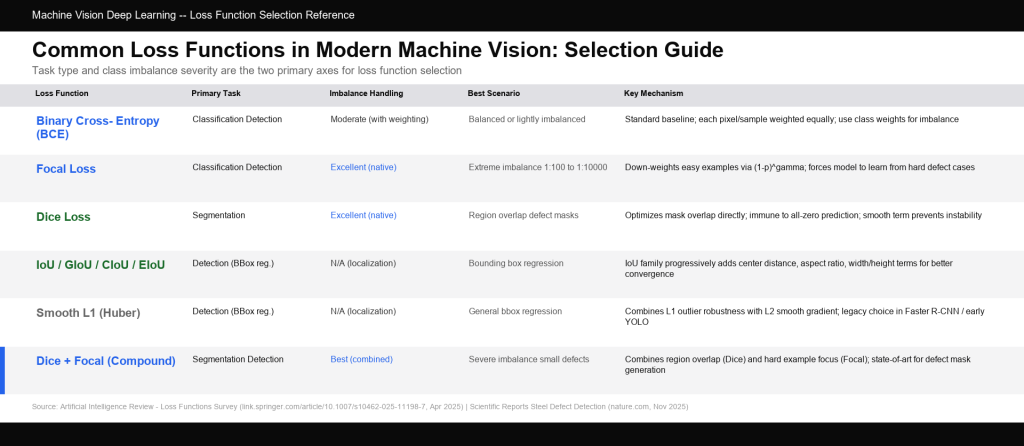
Loss function selection guide for machine vision tasks. Class imbalance handling and task alignment are the two primary selection axes. Compound losses combine strengths of multiple approaches.
IoU-Family Bounding Box Regression Losses
GIoU, CIoU, EIoU: Progressive Improvements for Detection
The vanilla IoU loss problem (vanishing gradient for non-overlapping boxes) led to a family of improved formulations that maintain gradient flow in all situations:
| Loss | Key Addition | Fixes |
| GIoU (Generalized IoU) | Enclosing box area term | Gradient for non-overlapping boxes |
| DIoU (Distance IoU) | Center point distance term | Faster convergence; center alignment |
| CIoU (Complete IoU) | Aspect ratio consistency term | Box shape convergence |
| EIoU (Efficient IoU) | Separate width/height terms + focal weighting | Faster convergence; handles small defects |
| SIoU (Spatial IoU) | Vector angle of offset direction | More coherent box drift during training |
In defect detection on manufactured parts — particularly for small defects like micro-cracks or pin misalignment — EIoU and CIoU have become the preferred regression losses. Research published in Scientific Reports (November 2025) on steel surface defect detection confirmed that “IoU-based loss functions have become mainstream, such as DIoU, CIoU, EIoU, and SIoU” for production defect detection pipelines, noting that these functions “significantly enhance localisation accuracy and convergence speed.”
Smooth L1 (Huber) Loss for Box Regression
Before IoU-family losses, Smooth L1 (Huber) loss was the standard bounding box regression loss. It behaves like L2 loss (squared error) for small residuals and L1 loss (absolute error) for large residuals — combining the smooth gradient of L2 with the outlier robustness of L1. It remains in use in architectures such as Faster R-CNN and many YOLO variants for the coordinate regression components.
Compound Losses: Combining Distribution and Region Signals
Dice + Focal + BCE: The Segmentation Triple
In high class-imbalance segmentation tasks — exactly the situation in AI defect mask generation — the best-performing loss functions are compound losses that simultaneously optimize at the distribution level (BCE/Focal) and the region level (Dice/IoU).
A compound loss commonly used in production inspection segmentation:
Total Loss = Dice Loss + λ₁·BCE Loss + λ₂·Focal Loss
Where λ₁ and λ₂ are weighting coefficients tuned on a held-out validation set. As documented in work published in arXiv on Unified Focal Loss, which proposes a hierarchical framework generalizing Dice and cross-entropy losses, the authors showed it is “robust to class imbalance and consistently outperforms other loss functions” across five imbalanced medical imaging datasets — results that translate well to industrial inspection scenarios with similar imbalance structure.
For teams building deep learning inspection models from scratch, the optimal compound loss configuration depends on the specific defect-to-background ratio, defect size distribution (smaller defects benefit more from focal loss), and boundary precision requirements. Training infrastructure that enables rapid loss function experimentation — paired with proper validation metrics (F1, mAP, mean IoU) rather than accuracy — is essential for effective tuning .
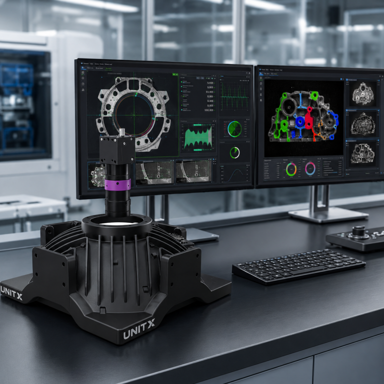
AI visual inspection platforms like UnitX CorteX achieve their reported 9× reduction in false rejection rates through, among other factors, sample-efficient training approaches that address the class imbalance problem at both the data level (via GenX synthetic defect generation) and the loss function level. The ability to train effective models from as few as 5 real defect images per defect type relies on this combined approach — it is not achievable with naive cross-entropy training on imbalanced data. For teams evaluating AI inspection platforms, UnitX customer case studies document concrete results across automotive, battery, and semiconductor production environments.
Evaluation Metrics vs. Loss Functions: An Important Distinction
Why You Should Not Train Directly on Accuracy
Accuracy (the fraction of correctly classified samples) is not a useful training loss because it is not differentiable — the gradient is zero almost everywhere except at the decision boundary. Loss functions (cross-entropy, focal loss, etc.) are differentiable proxies that enable gradient-based optimization while correlating with accuracy on balanced datasets.
In imbalanced inspection scenarios, accuracy is actively misleading as a metric. The correct evaluation metrics for inspection models are:
- Precision / Recall / F1-score — Explicitly measure defect detection performance independent of class size
- Mean Average Precision (mAP) — Standard for detection; accounts for both localization and classification accuracy across confidence thresholds
- Mean IoU (mIoU) — Standard for segmentation; measures average overlap across all classes
- False Acceptance Rate (FA) and False Rejection Rate (FR) — Industry-standard metrics in manufacturing quality control: FA measures defect escapes; FR measures overkill (good parts rejected)
Frequently Asked Questions
What loss function does YOLO use for defect detection?
YOLO architectures use a compound loss that combines: (1) classification loss (binary cross-entropy for each class) for the class prediction head; (2) objectness loss (BCE) for the confidence score; and (3) bounding box regression loss. In YOLOv5 and later, the regression loss uses CIoU or its variants. In YOLOv8 and YOLOv11, the classification head incorporates focal-style losses by default. Research on PCB defect detection using GBE-YOLOv8 (published March 2026) achieved 98.9% mAP@0.5 on PCB defect datasets using compound IoU-based and classification losses, demonstrating the effectiveness of this compound approach.
How do I choose gamma for focal loss in my inspection dataset?
Start with γ = 2 (the RetinaNet default) as a baseline. Then systematically evaluate γ values from 0.5 to 5 on your validation set, measuring recall on defect examples (not overall accuracy). The optimal gamma is the value that maximizes defect recall without excessively degrading precision. If your dataset has extreme imbalance (greater than 1:1000), start with higher values (γ = 3–4). If your defect samples are noisy or mislabeled, stay lower (γ = 1–2) to prevent the model from overfitting to difficult but incorrect examples.
Why is Dice loss better than BCE for segmentation?
BCE evaluates each pixel independently, which creates a class imbalance problem at the pixel level. Dice loss evaluates the entire predicted mask against the ground-truth mask jointly, so the model cannot minimize loss by predicting all background (all zeros). The Dice coefficient for an empty prediction against any non-empty ground truth is zero, producing maximum loss. This makes Dice loss naturally robust to class imbalance without requiring class weighting. However, Dice loss can be numerically unstable for very small or absent defects; the smoothing term (ε = 1e-6) in the denominator is essential.
What is the difference between IoU loss and Dice loss?
Both measure region overlap but differ in the denominator: Dice uses |Pred| + |GT| while IoU uses |Pred ∪ GT| = |Pred| + |GT| − |Pred ∩ GT|. Mathematically, Dice = 2×IoU / (1+IoU). In practice, the difference is small — both perform similarly in most segmentation tasks. Dice tends to be slightly more commonly used because its 0-to-1 range and its relationship to the F1-score (Dice coefficient = F1 score for segmentation) make it more interpretable.
Should I use a single loss function or a compound loss for my inspection model?
For severe class imbalance (the normal condition in industrial inspection), compound losses that combine distribution-level and region-level signals consistently outperform individual losses. The Dice + Focal combination is a well-validated starting point. The weighting coefficients (λ₁, λ₂) should be tuned on your validation set by measuring FA and FR rates on held-out defective samples — not overall accuracy. Investing in loss function tuning typically yields a 10–30% improvement in defect recall at equivalent false rejection rates, directly reducing escaped defects in production.